Search Results for: supervised machine learning

Train, Test And Validate Datasets In Machine Learning

The aim of this article is to help you understand the difference between testing, training and validating machine learning datasets.

Training Dataset

It is the dataset that we use to train an ML model. The model sees and learns from the training dataset.

Validation Dataset

The validation set is used to evaluate a particular model. This data is used by machine learning engineers to fine-tune the model’s hyperparameters. As a result, the model encounters this data on occasion, but never “learns” from it. The validation set findings are used to update the hyperparameters. Thus, the validation set influences a model indirectly.

Test Dataset

The test machine learning dataset serves as the gold standard for evaluating the model. It is only utilized when a model has been properly trained (using the validation and train sets). In most cases, the test set is utilized to compare rival models. In general, the test set is well-curated. It provides properly sampled data spanning the numerous classes that the model might face in the real world.

machine learning datasets

Importance Of Splitting

Supervised machine learning algorithm is about creating precise models which predict the target variable consistently with the inputs given to the model.

Now, carrying on with our learning related to machine learning datasets, there are multiple ways to measure the precision of your model. It depends on the kind of problem you are trying to solve. For regression, we may look at RMSE, absolute error, etc. For classification, we may look at precision, recall, etc.

We usually need unbiased evaluation to measure these properly, assess and validate the predictive performance. This means we cannot evaluate the predictive performance of the model with the same data that is used for training, hence we need fresh data that hasn’t been fed to the model. This can be accomplished by splitting the dataset.

How To Split Dataset Into Validation, Test And Train

We can simply use SKlearn’s module model_selection.train_test_split twice.

  • First, let’s split the data into train set and test set

X_train, X_test, y_train, y_test = train_test_split(X, y, test_size=0.2, random_state=42)

  • Second, split the train dataset again into train and validation

X_train, X_val, y_train, y_val  = train_test_split(X_train, y_train, test_size=0.25, random_state=42) (0.25 x 0.8 = 0.2)

Another Way To Split Dataset

train, validate, test = np.split(df.sample(frac=1), [int(.6*len(df)), int(.8*len(df))])

This will produce a 60%, 20%, 20% for training, test & validation, sets.

Summary

In this article you learned how to utilize SKlearn’s train test split(). You also learned that using data that hasn’t been used for model fitting is the best way to get an impartial estimate of the prediction performance of a machine learning model. Therefore, you must divide your dataset into different subsets.


References

The Best Books for Learning Data Science with Python in 2020

This article contains affiliate links. For more, please read the T&Cs.

Start (or continue) your data science journey here with these amazing books.

You may have heard the phrase “data is the new oil”. Regardless of your feelings about fossil fuels, it certainly contains in it more than a drop of truth.

It follows that if data is the new oil, data science is the engine that drives the new economy. In only a short time, data science has become arguably the hottest industry in the world, and it does not yet show any signs of slowing down.

One unique character of data science as a field is that there are many, varied pathways to become involved in it. Although a traditional path of a university degree is a great path to get into the industry, data science might also be one of the best fields for aspiring self-taught practitioners (after all, that’s why you are here!). Between free public datasets, cheap (often free) compute power and myriad of self-learning resources, all you need to teach yourself data science is some patience and commitment.

Having said that, we here at Data Courses understand that it can feel like there are too many resources out there and it can be overwhelming to decide where to start.

Not to worry. We’ve done the research and put together a shortlist of books that we think would get you well on your journey to becoming a data scientist. Take a look – also, many of the listed books are available for free!

Background Material – Statistics & Python

A solid grasp of statistics is highly recommended (if not absolutely mandatory) if you are looking to become a data scientist; and some programming proficiency is definitely required to follow most data science books out there. So, here we list material to help you either get a good grounding in data science (statistics), and with Python, which is our language of choice.

The Signal and the Noise: Why So Many Predictions Fail–but Some Don’t

This book by Nate Silver is now a classic. Silver gained fame as a political forecaster during the 2012 U.S. elections, before more recently going on to found the famous data-journalism website FiveThirtyEight

The appeal of The Signal and the Noise is in delivering examples of interesting prediction (i.e. modeling) case studies, that are objective, detailed yet approachable and digestible. This book is fantastic for helping the reader develop an intuitive understanding of how to use data to develop models the right way. There is a focus throughout the book on why models actually come out with the wrong predictions despite the mass amounts of data available to modelers.

Lessons that are covered in the book include:

  • Understanding that many economists and modelers in other fields try to predict outcomes too narrowly and are overconfident in their results
  • That models, as good as they can be, need to be reviewed by a human to ensure they’re not going awry
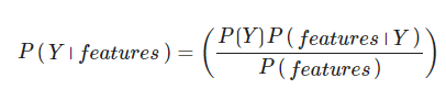
  • There are means of using Bayes’s theorem to understand how you can get errors in any models predictions

Available on Amazon.

Bayesian Methods for Hackers: Probabilistic Programming and Bayesian Inference

What does it mean to have 85% of observations indicate result X? Does it mean the same thing as there being an 85% chance of result X occurring? (hint: no)

Understanding of Bayesian methods are critical for data scientists. Yet, many books on Bayesian statistics can be inaccessible, and worse, boring. Which is unfortunate, because it is a fascinating subject. 

This book is written with programmers in mind. As a result, mathematics is kept to a minimum, and it provides plenty of examples along the way to develop your intuition. The book starts with an introduction to what Bayesian equations and math really mean for statistical analysis and how they can influence your work as well as the mathematics behind them. It then goes onto covering the PyMC Python library that is used throughout the book to provide practical examples in Python.

The book then goes on to cover the Law of Large Numbers and the Disorder of Small Numbers concepts to readers throughout the fourth chapter while providing many examples to help you get your head around the data. This is followed by an extensive chapter on loss functions and machine learning using Bayesian methods. The book is closed with a chapter on the concept of priors which leads into the last chapter on a very practical note examining A/b testing results using Bayesian methods.

Available for free here, and also on Amazon.

An Introduction to Statistical Learning

This book is written in the classical ‘textbook’ mold and is based on R, not Python. But don’t get us wrong; this is an excellent book.

Its visual and code examples definitely reduce the learning curve significantly in picking up the (admittedly dense) subject matter. 

It covers common and significant statistical methods for machine learning, such as linear regression, classification, tree-based methods, support vector machines, and clustering to name a few. The intro and first sections of the book cover statistical learning in detail along with some basic diagnostics and graphics you’ll need to know in any programming language (R or Python) to really dig into your data sets. As such, it is an excellent resource as a reference.

We also get a really strong understanding of resampling methods for model validation across regression and classification models. There are also sections covering polynomial and other types of regression to give us an understanding of non-linear modeling. The book then closes on two chapters around unsupervised learning, including methods of dimensionality reduction and clustering as well as extensive coverage of support vector machines (SVMs).

Or, if you are so inclined and have the patience, it is not a bad end-to-end read also, as far as these books go.

Available here.

Automate the Boring Stuff with Python

If you are new to Python (and new to programming), this is a solid starting point. On the one side of data science is statistical knowledge and on the other is knowledge of computer science, and that’s just where this book fits in. This is a book for beginners, but the author has done a great job in packing the book full of relatable, practical examples, rather than starting with hundreds of pages of unrelatable theory. They cover the Python Standard Library extensively as well as how to import other libraries for use within your scripting as well to build robust programs, all of which is extensible to data science as a discipline.

The resulting book is an easy, fast read that helps readers begin to appreciate the utility of programming while gaining familiarity with Python. 

Some of the examples like regular expressions, web scraping and dealing with csv/json files are also very useful for data science projects. The book includes details on how to perform many functions critical to understanding data flow and how to navigate many data types in Python. This includes searching for text in files across multiple files as well as how to create, update, move, and rename files and folders from Python itself. There is also an interesting set of examples of how to search the web and download website content to your local machine.

There is coverage of data management techniques involving Excel spreadsheets including formatting of Excel as well as some interesting coverage of managing PDF files, which may come in handy for a data scientist who is putting together a formal report for internal or external stakeholders. Some of the other functionality covered include how to send emails and text messages using Python, all of which come in handy when you’re up and running as a production data scientist or machine learning engineer that needs to monitor script and job performance along with your Data Engineers.

This book is likely to contain something for everyone.

Available here.

Data Science with Python

Python Data Science Handbook

This introductory data science book is for readers who may be familiar with Python but haven’t yet dealt much with data or who are looking to keep up with best practices. This is the best data science book on the subject to beginners we could think of.

I like the structure of this book. It starts the readers off with the fundamental tools for data analysis and manipulation in Numpy which is used for many mathematical functions and equations in Python. It then dives into Pandas which is a data management and manipulation library and is the most popular Python library in the Python ecosystem, something every data scientist using Python needs to be familiar with. There is then a full chapter on data visualization with Matplotlib, a skill that is very important in being able to convey complex data in graphical form when analyzing your data sets.

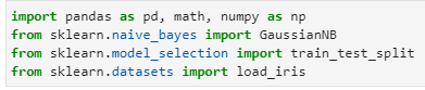
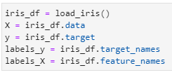
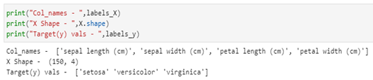
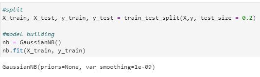
Then it goes on to practical overviews of various machine learning techniques, including examples and when they might be used. This section is really focused around an introduction of readers to the scikit-learn python library. They cover model tuning in detail as well as many machine learning models. This includes: Naive Bayes Classification, Linear Regression, Support Vector Machines, Decision Trees & Random Forests, Principal Component Analysis, K-Means, and a few other models.

From there the reader should be able to one for the next two books, having built a solid foundation. This is a book definitely worth checking out and is top of our list for getting your Python data science knowledge started.

Available here.

Deep Learning with Python

François Chollet is one of the creators of Keras, probably one of the top 2 or 3 machine learning interfaces in existence right now. One of Keras’ focus was on being a user-friendly machine learning framework, and this ethos shines through on Chollet’s book.

This book’s early pages cover the building blocks of machine learning theory without being overly mathematical, before moving on to practical, modern, examples and exercises in different fields. It also provides nice overviews of what deep learning as a concept truly is and what distinguishes it from traditional machine learning concepts in data science. There is extensive coverage of how to build neural nets and the mathematics behind them along with a section covering the fundamentals of machine learning, in case you didn’t read some of the earlier books.

Not only does it cover your simple regression/classification tasks, it also includes chapters on relatively complex subjects such as computer vision (and CNNs), texts (and RNNs), and even generative models (including GANs). 

Yes, the materials covered are vast and wide; but it somehow never feels overwhelming or rushed. 

Did I mention that this book is available here? Go get it.

Hands-On Machine Learning with Scikit-Learn, Keras, and TensorFlow

As the name suggests, Geron’s highly touted book is another that is focussed more on the practical than the theoretical. 

One difference between this book and Chollet’s is that its examples employ multiple packages; for instance easing the readers into machine learning with exercises using scikit-learn, before moving onto tensorflow for more complex models. 

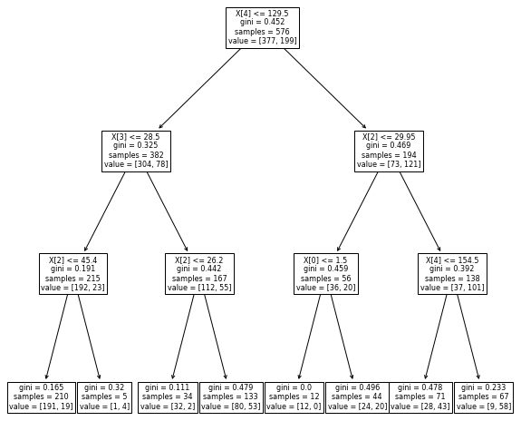
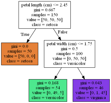
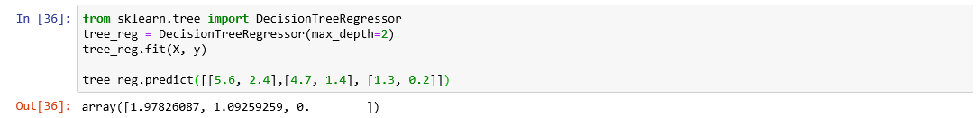
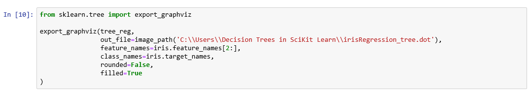
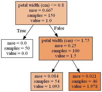
The book takes you on a guided example of a machine learning project using the scikit-learn library so you understand the full framework you’ll be working with in the future. You get to explore model development and training/testing of Support Vector Machines, Decision Trees, Random Forest, and ensemble methods. From there you dive into the TensorFlow library for Python and you learn how to build and train neural nets, architect them, and learn techniques for scaling models.

Geron has just updated the book and this second edition also covers Keras as a higher-level wrapper / interface for Tensorflow. 

Available on Amazon. Associated GitHub repo.

Natural Language Processing with Python

As they say, this is an oldie but a goodie. While some might argue (rightly) that the current approaches to machine learning with text have moved on somewhat, this is a great introduction to the field of natural language processing.

The book provides a mix of theoretical backgrounds in linguistics and computational linguistics as well as lots of practical examples with Python & NLTK, the classic language processing Library. As the book does not assume any Python knowledge, it is also well-suited for beginners. It starts with some basic domain knowledge about what natural language processing (NLP) truly involves and some of the jargon that goes with it. Then it jumps into how to process text using Python, a critical data crunching skill for data analysts and scientists alike.

The book progresses to more advanced topics such as analyzing grammar and sentence structure as well as the meaning of sentences as you get deeper into it. It ends on a chapter on managing linguistic data which walks through the high-level architecture of how you manage a corpus, or a large grouping of text (articles, etc.) and how that data is later manipulated to find insights.

Available on Amazon.

Deep Learning

Practical books are great, but for serious data science practitioners, a strong theoretical foundation might be just as important, especially in the long run. For those looking to shore up their understanding of the underpinning theories behind machine learning algorithms and processes, this book might be just right. 

This book is comprehensive in subject matter; guiding the reader by starting with the fundamental mathematics needed to progress throughout the book such as linear algebra and probability and information theory, before moving on to theory on more complex and topics such as regularisation, optimization, CNNs, RNNs. There is also deep and extensive coverage of practical methodologies and applications of deep learning to real-world problems.

There is also some detail at the end of the book regarding Monte Carlo Methods covering importance sampling, Markov Chains, and Gibbs Sampling.

It also expands the reader’s mind further than many books in that it devotes an entire section to state of the art research, which might be of interest once you’ve become comfortable with the more widespread techniques and practices.  What may be difficult about this book is that it spans over 599 pages in its hardcover format, but don’t be overwhelmed by its depth as you can always take the contents section by section as needed.

Available on Amazon

Bonus book – ML Strategy:

Machine Learning Yearning

This upcoming book by Andrew Ng is technically not available yet (it is in draft as of mid-Feb 2020), but a copy of it is accessible by signing up to a mailing list. Ng is as close a machine learning expert can be to a ‘celebrity’, having taught at Stanford, founded Coursera and now DeepLearning.ai. 

This book is aimed at those at managerial levels in organizations that are looking to implement data science / AI projects. As such, it focuses on high-level concepts and developing intuitive understandings of machine learning concepts and potential problems that may arise during a project. 

I think that practitioners can also find a lot of value in this book, though, whether it is for themselves or in improving their skills in communicating esoteric machine learning concepts to laypeople.

Available here (for now)

What’re you waiting for? Get out there and get reading the best data science books out there! If we have missed your favorites, let us know.

Ordinary Least Squares (OLS) Regression In Statsmodels

Today, we are going to learn about Ordinary Least Squares Regression in statsmodels. Some of you may know that linear regression is a supervised machine learning model that determines the linear relationship between the dependent (y) and independent variables (x) by finding the best-fit linear line between them.

When there is only one independent variable and the model must find the linear relationship between it and the dependent variable, a simple linear regression is used.

Here’s a Simple Linear Regression Equation, where bo denotes the intercept, b1 denotes the coefficient or slope, (x) denotes the independent variable, and (y) denotes the dependent variable.

The primary goal of a Linear Regression Model is to find the best fit linear line as well as the optimal intercept and coefficient values in order to minimize the error. The difference between the actual and predicted values is referred to as “error”, and the goal is to minimize it.

Assumptions of Linear Regression:

  1. Linearity: It states that the dependent variable (y) should be related to the independent variables linearly. A scatter plot between both variables can be used to test this assumption
  2. Normality: The (x) (independent) and (y) (dependent) variables should be normally distributed
  3. Homoscedasticity: For all values of (x), the variance of the error terms should be constant, i.e. the spread of residuals should be constant. A residual plot can be used to test this assumption
  4. Independence/No Multicollinearity: The variables must be independent of one another, with no correlation between the independent variables. A correlation matrix or VIF score can be used to test the assumption
  5. Error Terms: The error terms should be normally distributed. To examine the distribution of error terms, use Q-Q plots and Histograms. There should be no autocorrelation between the error terms. The Durbin Watson test can be used to determine autocorrelation. The null hypothesis is based on the assumption that there is no autocorrelation. The test’s value ranges from 0 to 4. If the test value is 2, there is no auto correlation

Let’s understand the methodology and build a simple linear regression using statsmodel:

  • We begin by defining the variables (x) and (y).
  • The constant bo must then be added to the equation using the add constant() method
  • To perform OLS regression, use the statsmodels.api module’s OLS() function. It yields an OLS object. The fit() method on this object is then called to fit the regression line to the data
  • The summary() method is used to generate a table that contains a detailed description of the regression results from pandas import DataFrame

dummy =  { ‘a’: [230.1,44.5,17.2,151.5,180.8,8.7,57.5,120.2,8.6,199.8,66.1,214.7,23.8,97.5,204.1,
                 195.4,67.8,281.4,69.2,147.3,218.4,237.4,13.2,228.3,62.3,262.9,142.9,240.1,
                 248.8,70.6,292.9,112.9,97.2,265.6,95.7,290.7,266.9,74.7,43.1,228],
           ‘cost’: [22.1,10.4,12,16.5,17.9,7.2,11.8,13.2,4.8,15.6,12.6,17.4,9.2,13.7,19,22.4,
                    12.5,24.4,11.3,14.6,18,17.5,5.6,20.5,9.7,17,15,20.9,18.9,
                    10.5,21.4,11.9,13.2,17.4,11.9,17.8,25.4,14.7,10.1,21.5]}
df = DataFrame(dummy,columns=[‘a’,’cost’])
df.head()
       

Ordinary Least Squares Regression

import statsmodels.api as sm
_a = df[[‘a’]]
_b = df[‘cost’]
a = sm.add_constant(_a) # adding a constant
#run a model
dummy_model = sm.OLS(_b, a).fit()

#predict
predict = dummy_model.predict(a)
print_model = dummy_model.summary()
print(print_model)

Ordinary Least Squares Regression

Let’s understand the summary report by dividing it into 4 sections:

SECTION 1:

Ordinary least squares regression

This section provides us with the basic details of the model that we can read and understand. Let’s take a look at: df (Residual) and df (Model Number). df is an abbreviation for “Degrees of Freedom”, which is the number of independent values that can vary in an analysis.

In regression, residuals are simply the error rate that is not explained by the model. It is the measurement of the distance between the data point and the regression line.

df(Residual) can be calculated as:

Where n is number of records, k is df(model).

SECTION 2:

Ordinary least squares regression

R squared: The degree to which the dependent variables in (x) explain the variation in the dependent variable (y). In our case, we can say that 81.1% variance is explained by the model. The disadvantage of an R2 score is that as the number of variables in x increases, R2 tends to remain constant or even increase by a small amount. The new variable, on the other hand, may or may not be significant.

Adj. R square: This overcomes the disadvantage of the R2 score and is thus considered more reliable. Adj. R2 does not consider variables that are “not significant” for the model.

F statistic = Explained variance / unexplained variance.

The Fstat probability is lower than 0.05(alpha value). It means that the probability of getting 1 coefficient to be non zero is 2.44e-15.

Log-Likelihood: The maximum likelihood estimator is derived from the likelihood value, which is a measure of fit/goodness of model.

AIC and BIC: These 2 methods are used for scoring and selecting models.

SECTION 3:

Ordinary least squares regression

The column coef is the value b1.

Std err is the error of each variable (distance away from regression line)

T and P>|t| are the tstat values.

[0.025,0.975] – 5% alpha/95% confidence interval range, if coef value is in between this, it is called acceptance region.

SECTION 4:

Ordinary least squares regression

Omnibus: It determines whether the explained variance in a set of data is significantly greater than the unexplained variance in the aggregate. We hope that the Omnibus score is close to 0 and the probability is close to 1, indicating that the residuals follow normalcy.

Skew: It is a measure of data normalcy. It also drives omnibus and we the value of skew should be close to 0.

Kurtosis: Is a measure of curvature of data.

Durbin-Watson Test: Test is used to autocorrelation in the data.

JB and prob(JB): Is used to test the normality of data.

Cond no: Is used to check collinearity in the data.

Summary

To summarize, you can think of ordinary least squares regression as a strategy for obtaining a ‘straight line’ that is as close to your data points as possible from your model. Although OLS is not the only optimization strategy for this type of task, it is the most popular because the regression outputs (that is, coefficients) are unbiased estimators of the true values of alpha and beta.


References

Learn About Core Features Of Scikit-learn

In the realm of artificial intelligence (AI), scikit-learn is a prominent open-source and machine learning (ML) library. Classification, regression, clustering, and dimensionality reduction are just a few of the useful tools in the scikit-learn toolkit for ML and statistical modelling. In this tutorial, you will learn about scikit-learn features.

Scikit-learn is primarily written in Python, while several fundamental algorithms are written in programming language Cython to increase efficiency. Scikit-learn also works with a variety of other Python libraries, including graphing libraries Matplotlib, pandas DataFrames, NumPy for array vectorization, Plotly, Scipy, etc.

Scikit-learn Library” has many important features, and some of them are listed below:

  • Supervised Models: A training set is used in supervised learning to teach models to produce the desired output. This training dataset contains both correct and incorrect outputs, allowing the model to learn over time. The loss function is used by the algorithm to measure its accuracy, and it adjusts until the error is sufficiently minimized. Example: Linear regression, random forest, XGBoost, etc.
  • Datasets: Scikit-learn includes a few small standard datasets that do not require the download of any files from a third-party website. Example: load_iris()  and load_diabetes() are some in-built datasets to practice on.
  • Parameter Tuning: Hyperparameter optimization is the process of conducting a search to find the set of specific model configuration parameters that result in the model’s optimal performance on a certain dataset.
  • Feature Selection: Feature selection is a technique for reducing variables by using specific criteria to select the variables that are most useful in the dataset which can help to predict the target in the model. Example: “VarianceThreshold” feature selection, univariate feature selection with SelectKBest, recursive feature elimination (RFE) and feature selection sequential feature selection (SFS).
  • Dimensionality Reduction: Dimensionality reduction is an unsupervised machine learning strategy that selects a collection of important features to reduce the number of feature variables for each data sample. Example: Backward Feature Elimination, principal component analysis, etc.

Feature selection is similar to dimensionality reduction in that the goal is to reduce the number of features, but both are fundamentally different. The distinction is that feature selection allows you to decide which features to keep or delete from the dataset. Dimensionality reduction, on the other hand, leads to the projection of data that ends in new input features.

  • Cross-validation: Cross-validation is a method of testing ML models that involves the training various models on subsets of the available input data and then assessing them on the complementary subset. Overfitting, or the failure to generalize a pattern, can be detected using cross-validation.
  • Ensemble Methods: Ensemble methods is basically a technique for developing multiple models and then combining the latter to get better results. Usually, ensemble methods produces more accurate results. Example: random forest, AdaBoost, GBM, etc.
  • Feature Extraction: The feature extraction module can be used to extract features in a format that machine learning algorithms can understand from datasets that include formats such as text and images.
  • Clustering: Cluster analysis, or clustering, is a sort of unsupervised machine learning paradigm. It discovers natural grouping in data automatically. Unlike supervised learning (such as predictive modelling), clustering algorithms just evaluate the incoming data and look for natural groups or clusters in feature space. Example: k-means clustering.

(I prefer using scikit-learn since it provides a lot of versatility. The official documentation includes many examples. In the next half of this article, I’ll show you some of the scikit-learn library’s more impressive features that you may not be aware of.)

1.   Plot The Decision Tree

The “Plot Tree Function” can be used to illustrate a decision tree model. Plot function lets you add feature names with a parameter, “feature_names”.

from sklearn.tree import plot_tree

2.   Dummy Features

If you want to generate dummy features in a dataset with a particular value, you can do that by using the “Add Dummy Feature” built-in in the scikit-learn library.

from sklearn.preprocessing import add_dummy_feature

3.   Impute Missing Values with Iterative Imputer

To replace (impute) missing values in datasets, we usually employ straightforward methods. For numerical features, these methods are mean/median, and for categorical features, mode is one of the methods that can be used. Advanced approaches such as IterativeImputer are also available. IterativeImputer employs a machine learning model like BayesianRidge to estimate missing values based on all attributes in your dataset. This indicates that the dependent variable will be the feature with missing values, while the other characteristics will be independent variables.

from sklearn.impute import IterativeImputer

4.   Identify Estimators As Regressors/ Classifiers

With two simple functions in the scikit-learn library, you can tell if a model solves a regression/ classification task. “is_classifier” and “is_regressor” are two functions that can be used to determine whether something is a classifier or a regressor.

from sklearn.base import is_regressor
from sklearn.base import is_classifier

5.   Cross-Validation And Prediction

You may use scikit-cross learn’s val predict function to perform cross-validation and prediction for the estimator.

from sklearn.model_selection import cross_val_predict

6.   Pick Important Features Using SelectFromModel

When running a model, all the features are not important. You may use the “SelectFromModel Function” to find and pick important features for your model. SelectFromModel just drops less crucial features based on a specified threshold, that is why it is less resilient.

from sklearn.feature_selection import SelectFromModel

7.   RandomizedSearchCV (hyperparameter tuning)

The function RandomizedSearchCV trains and evaluates multiple models by selecting a random number of hyperparameter distributions from a predefined list. After training numerous versions of the model with randomly chosen combinations of a hyperparameter, the function selects the most successful version with the best set of parameter values.

from sklearn.model_selection import RandomizedSearchCV

8.   Load Text Files

You can use the load files function in scikit-learn to load text files. Every folder within the main/root folder will be treated as a separate category by the load files, and all docs within the same folder will be assigned to that specific category.

from sklearn.datasets import load_files

9. Determine Target Data Type

We have independent variables and the targeted variable when working with supervised ML Mode. To decide whether to solve a problem using regression or classification, we need to know what type of data is the target variable (Y). The target variable’s type of data can be determined using the function type of target.

from sklearn.utils.multiclass import type_of_target

Summary

Scikit-learn is one of the most popular ML libraries. It has all the features which can be used to create an end-to-end ML solution. You may also utilize scikit-learn in your machine learning project and apply some of its lesser known capabilities as explained in this article.


References

Official documentation for:

What Is Scikit-learn?

Scikit-learn/Sklearn (formerly scikits. learn) is perhaps Python’s most useful machine learning (ML) library. Regression, dimensionality reduction, classification and clustering are only a few of the useful methods in the “Sklearn Library” for statistical modeling and for creating ML models.

Origin Of Scikit-learn

Data scientist David Cournapeau created the open source scikit-learn package as a Google Summer of Code Project. Later, Matthieu Brucher joined the project and began using it as part of his thesis research. The French national research institution, the National Institute For Research in Digital Science and Technology (Inria) became involved in 2010, and the first public update (v0.1 beta) was released in late January 2010.

Inria, Google, French company Tinyclues, and the Python Software Foundation have all contributed to the project financially, and it has over 30 active contributors today.

Some Components

  • Supervised learning algorithms: Consider any supervised machine learning algorithm you’ve heard of; chances are it’s included in scikit-learn. The scikit-learn toolbox includes everything, from linear regression to Stochastic Gradient Descent (SGD), decision tree, random forest, etc. One of the main reasons for scikit-learn’s popularity is the development of ML algorithms. Here are a few examples:
    • Random forest
    • Decision tree
    • Ridge regression
  • Unsupervised learning algorithms: Once again, the offering includes a wide range of machine learning algorithms ranging from principal component analysis (PCA), clustering, unsupervised neural networks and factor analysis
  • Cross-validation: There are various methods for testing the accuracy of supervised models on unseen data using Sklearn
  • Clustering: It is an unsupervised learning technique that automatically groups related objects into sets. Few examples:
    • K-means
    • Mean shift
    • Spectral clustering
    • Hierarchical clustering
  • Dimension reduction: The method of reducing the number of random variables is known as dimensionality reduction. Few examples:
    • Principal component analysis
    • Non-negative matrix factorization (NMF)
    • Feature-selection techniques

Model selection is the action of comparing, validating, and selecting parameters and models. It utilizes algorithms such as grid search, cross-validation, and metric functions. Scikit-learn provides all the demonstrable algorithms and methods in easily accessible APIs.

  • Data preprocessing: One of the first and most critical steps in the machine learning process is the preprocessing of data, which includes features extraction and normalization. Normalization converts features into new variables, usually with a zero mean and a unit variance, but often with a value between a given minimum and maximum, usually 0 and 1. Feature extraction converts text or photographs into numbers that can be used in machine learning
  • Feature selection: It is used to define useful attributes for creating supervised models
  • Various dummy datasets: This is useful when studying scikit-learn. You can practice machine learning on different datasets provided (ex- IRIS dataset). Having them on hand while studying a new library is extremely beneficial
  • Parameter tuning: It is used to get the best out of supervised models
  • Manifold learning: This is a technique for summarizing and envisioning complex multidimensional data

Why Use Scikit-learn In Machine Learning

Scikit-learn is both, well-documented and straightforward to learn/use if you want an introduction to machine learning, or if you want the most up-to-date ML testing tool. It lets you construct a predictive data model with a few lines of code and then apply that model to your data as a high-level library. It’s flexible and integrates nicely with other Python libraries such as Matplotlib for charts, Numpy for numerical computations, and Pandas for DataFrames.

Scikit-learn contains many supervised & unsupervised learning algos. Most importantly, it is by far the simplest and cleanest ML library. It was created with a software engineer’s perspective. Its central API architecture revolves around being simple to use while still being versatile and flexible for research endeavors. Because of its robustness, it is suitable for use in any end-to-end ML project — from research to production deployments. It is based on the machine learning libraries mentioned below:

NumPy: is a Python library that allows you to manipulate multidimensional arrays and matrices. It also includes a large set of mathematical functions for performing various calculations

SciPy: is an environment of libraries for performing technical programming tasks

Matplotlib: is a library that can be used to build different charts and graphs

(Tip: Please do refer to the Andreas Mueller (one of the main scikit-learn contributor) cheat sheet for machine learning. It is a very effective representation for comprehending the scope of Scikit’s ML algorithms.)

Overview Of Few Machine Learning Algorithms

  • Linear regression: The relationship between two factors is shown or predicted using linear regression models. The factor being predicted is known as the “dependent variable”. The “independent variables” are the factors that are used to predict the value of the dependent variable. Each observation in linear regression has two values. One of them represents the dependent, while the other means the independent variable. In this basic model, a straight line approximates the relationship between both the variables.
  • Logistic regression: Logistic regression is another statistical methodology that machine learning has borrowed. It’s the form of choice for binary classification issues (problems with two class values). Like linear regression, the purpose of logistic regression is to find the values for the coefficients that weigh each input variable. In contrast to linear regression, the output estimate is transformed using a non-linear function known as the logistic function.
  • Decision trees: It is a popular form of ML algorithm, and often used in predictive modeling. Decision tree model is often described as a binary tree. The latter is made up of data structures and algorithms. A split on a single variable (z) is represented by each node (variable should be numeric). Output variable (y) is used to make a prediction. Predictions are made by processing through the tree’s splits before reaching a leaf node; then outputting the class value at the node. Trees are very fast to learn and even faster to predict.
  • Random forest : It is a set of decision trees. Each tree is categorized, and the tree “votes” for that class to classify a new object based on its attributes. The classification with the most votes is chosen by the forest (overall, the trees in the forest).

Here’s how each tree is planted and grown:

If the training set contains X cases, a sample of X cases is selected at random. This sample will serve as the tree’s training package.

Let’s assume A input variables, a number y less than A is set down so that variables are randomly picked from input dataset at each node, and the best split on y is used to split the node further. y’s value is kept constant.

Now, each tree is grown to its full potential.

  • Gradient boosting algorithm : These are boosting algorithms that are used when large amounts of data must be processed to make accurate predictions. Boosting is an ensemble learning algorithm that improves robustness by combining the predictive strength of many base estimators. To put it another way, it combines many weak or average predictors to create a good predictor.

Let’s Build A Simple Machine Learning Model

Consider a simple scenario wherein you must determine, based on the weather, whether to bring an umbrella or not. You have access to the training data (temperature). Your mind makes a relation between the input (temperature) and the output (temperature) (take an umbrella/not).

Now, let’s move on to an algebraic problem where the model will predict the results for us:

  • Generate the dataset – Focus on the equation passed in the dataset creation.
What is scikit learn

#load libraries
import numpy as np, pandas as pd
from random import randint
limit_train = 200
count_train = 10
inp = list()
out = list()
for i in range(count_train):
    _a = randint(0, limit_train)
    _b = randint(0, limit_train)
    _c = randint(0, limit_train)
    _d = randint(0, limit_train)
    equation = _a + (1/2*_b) + (5/3*_c)+ 2*_d
    inp.append([_a, _b, _c, _d])
    out.append(equation)

  • Model training – Now that we have the training data, we can build a Linear Regression Model and feed it the training data.
What is scikit learn

from sklearn.linear_model import LinearRegression
predictor = LinearRegression(n_jobs=-2)
predictor.fit(X=inp, y=out)

  • Pass the test data set : Lets pass the test data as 1,2,3,4.

As per the equation the output should be:

1 + (1/2)*2 + (5/3)*3 +2*4= 15

What is scikit learn

test = [[1, 2, 3, 4]]
result = predictor.predict(X=test)
coeff = predictor.coef_
print(‘Outcome : {}\nCoeff : {}’.format(result, coeff))

As the above model had access to the training data, it determined the weights and the inputs to produce the needed output. When test data was passed, it got the correct response.

Summary

This was a high-level introduction to one of Python’s most efficient and adaptable machine learning libraries. Sklearn, that started out as a Google-led project, has not only determined the way models are written, but it has also broken new ground in Python for machine learning, sculpting the language and, to some degree, the ecosystem. Because of this, Sklearn’s outcome on science, ML, and automation gains importance.


References

Dimensionality Reduction Using scikit-learn in Python

This article contains affiliate links. For more, please read the T&Cs.

Datasets with a large number of features are very difficult to analyze. Besides, the amount of computational power that you might need for such a task would be very big. Dimensionality reduction offers a powerful way of dealing with high dimensional data. Dimensionality reduction techniques help us to reduce the dimension of the feature set, without losing much information allowing for robust analysis. Additionally, it can keep, or even improve, the performance of a model generated from the simplified data.

In this article, we present to you a comprehensive guide to three dimensionality reduction techniques. They are available in the scikit-learn library in Python.

Dimensionality Reduction

High-dimensional data presents a challenging task for statistical models. Luckily, much of the data is redundant and can be reduced to a smaller number of variables. It’s possible to do it without losing much information.

Normally, we use dimensionality reduction in machine learning and data exploration. In machine learning, we use it to reduce the number of features. This will decrease the computational power and possibly lead to a better performance of the model.

Similarly, we can use dimensionality reduction to project data into two dimensions. Such visualization can help us to detect outliers or clusters of data.


Principal Component Analysis (PCA)

PCA is the most practical unsupervised learning algorithm. It’s inherently a dimensionality reduction algorithm. If your data has more than 3 dimensions, you can visualize it by using PCA.

PCA projects the data on k orthogonal bases vectors u that minimize the projection error. For instance, let’s say that we have a 2D dataset that has features height and weight. By using PCA we can project this 2D dataset to 1D using the vector u.

An Illustration of the Principal Component Analysis projection
Principal Component Analysis Illustration

When we apply PCA to a dataset, it identifies the principal components of data. Such attributes account for the most variance in the data. Moreover, PCA always leads to components that are orthogonal.


When should you use PCA? 

It’s important to note that PCA works well with highly correlated variables. If the relationship between variables is weak, PCA won’t be effective. You can look at the correlation matrix to determine whether to use PCA. If most of the coefficients are smaller than 0.3, it’s not a good idea to use PCA.

Additionally, you can look at the correlation coefficients to determine which variables are highly correlated. If you find such variables, you can use only one of them in the analysis. A cut off for highly correlated is usually 0.8.


Linear Discriminant Analysis (LDA)

LDA is a supervised machine learning algorithm. It is most commonly used for dimensionality reduction. The general LDA approach is similar to PCA. LDA finds the components that maximize both the variance of the data and the separation between multiple classes. We often use LDA in preprocessing for classification models.

When should you use LDA?

We can use LDA only for supervised learning. This means that we need to know the class labels in advance.

Some experiments compared classification when using PCA or LDA. These experiments show that classification accuracy tends to improve when using PCA. Finally, the performance of these techniques largely depends on the characteristics of the dataset.


t-distributed Stochastic Neighbouring Entities (t-SNE)

t-SNE is a valuable data visualization technique. It is unsupervised and non-linear. t-SNE has a cost function that is non-convex. Therefore, different initializations can lead to different local minima. If the number of features is very high, it is advised to first use another technique to reduce the number of dimensions.

When should you use t-SNE?

t-SNE places neighbors close to each other, so we cannot clearly see how the samples relate with respect to their features. It is used for data exploration, especially for visualizing high-dimensional data.

t-SNE does not learn a function from the original space to the new one. Because of this, it cannot map the new data according to the previous t-SNE results. In other words, it cannot be used in classification models.


Hands-on Example With the Iris Dataset

In this paragraph, we will show you how to use dimensionality reduction in Python. Firstly, let’s import the necessary libraries, including Pandas and Numpy for data manipulation, seaborn and matplotlib for data visualization, and sklearn (or scikit-learn) for the important stuff.

import pandas as pd
import numpy as np
import matplotlib.pyplot as plt
import seaborn as sns
from mpl_toolkits.mplot3d import Axes3D
from sklearn import datasets
from sklearn.decomposition import PCA
from sklearn.discriminant_analysis import LinearDiscriminantAnalysis
from sklearn.preprocessing import StandardScaler
from sklearn.manifold import TSNE

Secondly, we need to import a dataset. We chose the Iris dataset.

# import the iris dataset
iris_dataset = datasets.load_iris()
X = iris_dataset.data 
y = iris_dataset.target
target_names = iris_dataset.target_names

Thirdly, let’s take a look at the dataset that we will use. We chose Iris dataset because it’s a well-known dataset in machine learning literature. It contains 3 classes, where each class refers to a type of Iris plant.

iris_df = pd.DataFrame(iris_dataset.data, columns = iris_dataset.feature_names)
iris_df['Species']=iris_dataset['target']
iris_df['Species']=iris_df['Species'].apply(lambda x: iris_dataset['target_names'][x])
iris_df.head()
Information about Iris dataset

We can also see how classes are separated regarding different features.

colors = {'Setosa':'#FCEE0C','Versicolor':'#FC8E72','Virginica':'#FC3DC9'}

#Let see how the classes are separated regarding different featueres

sns.FacetGrid(iris_df, hue="Species", height=4, palette=colors.values()) \
   .map(plt.scatter, "sepal length (cm)", "sepal width (cm)") \
   .add_legend()


sns.FacetGrid(iris_df, hue= "Species", height=4, palette=colors.values()).\
map(plt.scatter, "petal length (cm)", "petal width (cm)").add_legend()
plt.show()
Visualization of the Iris dataset considering only two features at the time

A correlation matrix can help us understand the dataset better. It tells us how our four features are correlated. The correlation matrix is easily obtained by using the seaborn library. Here you can check out our tutorial on different plots that you can create with seaborn.

Correlation matrix of Iris dataset

From the correlation matrix, we can notice a high correlation score between features Sepal Length and Sepal Width.

PCA with 2 components

Now, let’s apply PCA with 2 components. This will help us represent our data in two dimensions.

First, we need to normalize the features.

#Use standard scaler to normalize the features
scaler = StandardScaler()
X = scaler.fit_transform(X)

After the normalization, we can transform our features using PCA.

pca2 = PCA(n_components=2)
X_r = pca2.fit_transform(X)

for color, i, target_name in zip(colors.values(), [0, 1, 2], target_names):
    plt.scatter(X_r[y == i, 0], X_r[y == i, 1], color=color, alpha=.8, 
                label=target_name, s=130, edgecolors='k')
plt.legend(loc='best', shadow=False, scatterpoints=1)
plt.xlabel('1st PCA component')
plt.ylabel('2nd PCA component')
plt.title('PCA of IRIS dataset')

# Percentage of variance explained for each components
print('explained variance ratio (first two components): %s' # First two PCA components capture 0.9776852*100% of total variation!
      % str(pca2.explained_variance_ratio_))

plt.show()

PCA with 2 components helped us easily plot our dataset in two dimensions.

PCA with two components helps us to visualize Iris dataset

We can see that Iris Setosa is very different from the other two classes. Also, we can calculate the explained variance. The explained variance will tell us how much of variance do our two components take up.

We got a result of 95.8%, as a total for the first two components. This means that the first two principal components take up 95.8% of the variance. This is a good result and it means that our 2D representation is meaningful. If this score was less than 85%, it would mean that our 2D representation of data might not be valid.

PCA with 3 components

To get a better understanding of the interaction of the features, we can plot the first three PCA components.

fig = plt.figure(1, figsize=(8, 6))
ax = Axes3D(fig, elev=-150, azim=110)
pca3 = PCA(n_components=3)

X_reduced = pca3.fit_transform(iris_dataset.data)
ax.scatter(X_reduced[:, 0], X_reduced[:, 1], X_reduced[:, 2], c=y,
           cmap=plt.cm.spring, edgecolor='k', s=130)
ax.set_title("First three PCA components")
ax.set_xlabel("1st PCA component")
ax.w_xaxis.set_ticklabels([])
ax.set_ylabel("2nd PCA component")
ax.w_yaxis.set_ticklabels([])
ax.set_zlabel("3rd PCA component")
ax.w_zaxis.set_ticklabels([])

# Percentage of variance explained for each component
print('explained variance ratio (first three components): {}' # First three PCA components capture 0.99478781 of total variation!
      .format(pca3.explained_variance_ratio_))

plt.show()
Iris dataset represented with the first three principal components


LDA with two components

Now let’s calculate the first two LDA components and visualize them. In both PCA and LDA, the Setosa data is well separated from the other two classes. Also, we can see that LDA performs better at keeping the overlap between Versicolor and Virginica to a minimum.

lda = LinearDiscriminantAnalysis(n_components=2)
lda.fit(X, y)
X_r2 = lda.transform(X)
plt.figure(figsize=(10,8))
for color, i, target_name in zip(colors.values(), [0, 1, 2], target_names):
    plt.scatter(X_r2[y == i, 0], X_r2[y == i, 1], alpha=.8, color=color,
                label=target_name,  s=130, edgecolors='k')
plt.legend(loc=3, shadow=False, scatterpoints=1)
plt.xlabel('LDA1')
plt.ylabel('LDA2')           

plt.title('Iris projection onto the first 2 linear discriminants')

print('Explained variance ratio (first two linear discriminants): {}'.format(lda.explained_variance_ratio_))
plt.show()
Iris dataset projected with first two linear discriminants

t-SNE

We will visualize our dataset using t-SNE. We set the dimension of the embedded space to two.

tsne = TSNE(n_components=2, n_iter=1000, random_state=42)
X_tsne = tsne.fit_transform(X)

figure = plt.figure
figure(figsize=(10, 8))

for color, i, target_name in zip(colors.values(), [0, 1, 2], target_names):
    plt.scatter(X_tsne[y == i, 0], X_tsne[y == i, 1], alpha=.8, color=color,
                label=target_name,  s=130, edgecolors='k')
plt.legend(loc='best', shadow=False, scatterpoints=1)
           
plt.title('Iris projection onto the first 2 linear discriminants')
plt.show()
t-SNE projection with 2 dimensions

This is already a significant improvement over the PCA and LDA. As you can see, Iris species form very clear clusters.

Summary

In this post, we covered the fundamental dimensionality reduction techniques in Python using the scikit-learn library. They helped us to reduce the number of dimensions in our original dataset and to visualize our data. We uncovered some hidden relationships between our features.

In the table below we give an overview of the techniques that we explored.

Summary of the dimensionality reduction techniques


We encourage you to further study this topic. All the code from this article you can find in our Github repository. And, in conclusion, we recommend several sources of information: 

Naive Bayes Classifier in Scikit-learn

Before jumping into the details of Naive Bayes Classifier, let’s first understand what a classifier is.

The Classification Algorithm is a supervised learning technique that uses training data to determine the category of new observations. Classification is the process of machine learning (ML) from a dataset or observations, and then classifying fresh observations into one of several classes or groupings. Yes or No, 0 or 1, Spam or Not Spam, Cat or Dog, are such examples. Targets/labels or categories are all terms that can be used to describe classes.

There are two types of classifications:

  • Binary Classifier: This type of classifier is used when there are only two possible outputs to a classification task. Example – Yes/No, Male/Female, Spam/Not Spam, and so on
  • Multi-class Classifier: A Multi-class Classifier is used when a classification task involves more than two outcomes. Example – Classifications of different types of music, etc

Some types of ML classification algorithms:

What is Naive Bayes Classifier?

The Bayes Theorem is used to create a statistical classification approach known as Naive Bayes. It’s one of the most basic supervised learning algorithms out there. The Naive Bayes Classifier is a reliable, accurate and fast algorithm. On large datasets, it has great accuracy and speed.

The Naive Bayes Classifier implies that the influence of one characteristic in a class is independent of the effect of other features. For example, a loan applicant’s worth is determined by his or her income, prior loan, transaction history, age, and geography. Even though these traits are interrelated, they are nonetheless evaluated separately. Because this assumption makes calculation easier, it is regarded as naive. Class conditional independence is the term for this assumption.

Naive Bayes Classifier
  • P(h): prior probability of h
  • P(h|D): posterior probability
  • P(D): prior probability of predictor
  • P(D|h): It is the likelihood which is the probability of predictor given class

Different Kinds Of Naive Bayes Classifiers

  • Gaussian Naive Bayes – The data from each label is assumed to be derived from a simple Gaussian distribution using the Gaussian Naive Bayes classifier
  • Multinomial Naive Bayes – The characteristics are assumed to be chosen from a basic Multinomial distribution
  • Bernoulli Naive Bayes – The model assumes that the features are binary (0s and 1s) in nature. Text classification with the ‘bag of words’ model is an application of Bernoulli Nave Bayes classification
  • Complement Naive Bayes – It was created to correct the Multinomial Bayes classifier’s severe assumptions. This type of NB classifier works well with unbalanced data sets

Building Naive Bayes Classifier

We can build a simple Naive Bayes Classifier using scikit-learn as shown below:

  • Loading needed libraries:

import pandas as pd, math, numpy as np
from sklearn.naive_bayes import GaussianNB
from sklearn.model_selection import train_test_split
from sklearn.datasets import load_iris

Naive Bayes Classifier
  • Let’s load one of the inbuilt datasets in sklearn library:

iris = load_iris()
X = iris.data
y = iris.target
y_labels = iris.target_names
X_labels = iris.feature_names

  • Let’s look at variables:

print(“Col_names – “,labels_X)
print(“X Shape – “,X.shape)
print(“Target(y) vals – “,labels_y)

  • Let’s split the data and fit the data:

#split
X_train, X_test, y_train, y_test = train_test_split(X,y, test_size = 0.2)
#model building
nb = GaussianNB()
nb.fit(X_train, y_train)

Naive Bayes Classifier
  • Let’s evaluate the model using test data:

nb.score(X_test, y_test)

The simple Naive bayes has performed well with a score of 0.9

Summary

Pros:

  • Predicting the test dataset’s class is simple and quick. It’s also good at multi-class prediction
  • When the assumption of independence is true, a Naive Bayes classifier outperforms other models such as logistic regression, and it requires less training data
  • When compared to numerical input variables, it performs well with categorical input variables (s)

Cons:

  • If a categorical variable in the test dataset has a category that was not included in the training data set, the model will assign a probability of 0 and will be unable to generate a prediction. This is called  “Zero Frequency.” We can use  Laplace estimation as a way to avoid this issue. Laplace estimation is one of the basic smoothing techniques out there
  • The assumption of independent predictors is another flaw in Naive Bayes since in real life, getting a collection of predictors that are totally independent is nearly impossible

References

Building Decision Tree Using Scikit-learn

“Decision Tree” is a type of supervised learning machine learning algorithms family which can solve both, regression and classification problems. Decision trees machine learning is to construct a training model that can be used to predict the target variable’s class or value by learning the basic decision rules from prior data (training data). To be more specific, a decision tree is a type of a probability tree that helps make a decision about a kind of a process.

When using this algorithm to predict a record’s class label, we must start at the top of the tree. The root & record attributes are compared. Based on this, we follow the branch that corresponds to that value and then move on to the next node. A decision tree is used in many real life situations such as business, and even engineering.

Types of Decision Trees

There are 2 types of decision trees based on the target variable:

Categorical Variable: Where the target (y) variable is categorical

Continuous Variable: Where the target (y) variable is continuous

Components of Decision Trees

  • Root node: Symbolizes the total sample, which is then separated into two or more homogeneous groups
  • Parent  & child nodes: A parent node of sub nodes is a node that is divided into sub nodes, whilst sub nodes are the “children” of a parent node
  • Decision node: Formed when a sub node splits into more sub nodes
  • Splitting: Is the method of splitting a node into two/more sub nodes
  • Pruning: Is the method of eliminating sub nodes from a decision node
  • Terminal / Leaf nodes: These are the nodes that do not split
  • Sub-Tree  / Branch: A sub-tree/branch is a part of the tree
Decision tree machine learning

Assumptions While Creating A Decision Tree

Here are a few assumptions made while creating a decision tree:

  • At first, a complete training dataset is regarded as the root
  • Basis attribute values and records are dispersed recursively
  • Using some statistical approaches (such as those listed below), it is possible to place attributes as the tree’s root or internal node

How To Select An Attribute As Root Node

Choosing the attribute to insert at the root / at different levels of decision tree as internal nodes is a complex step since the dataset contains multiple features (variables). The problem cannot be solved by selecting any node at random as the root because it may end up with low accuracy & poor results.

This is solved by utilizing an algorithm such as Gini index, information gain, etc. Every attribute’s value will be calculated using these algorithms. The values are sorted, and characteristics are ordered in the tree, with the attribute having the highest value at the top (in the case of information gain).

Building Simple Decision Tree (Classification) Model Using Scikit-learn

We’ll using a dataset from Kaggle – Diabetes.

Download the .csv files and load them into the Jupyter environment.

Data Dictionary:

Data Import:

decision tree machine learning

import pandas as pd, numpy as np
df = pd.read_csv(‘diabetes.csv’)
df.head(2)

Feature Selection:

feature = [‘Pregnancies’, ‘Insulin’, ‘BMI’, ‘Age’,’Glucose’,’BloodPressure’,’SkinThickness’,’Insulin’]
X = df[feature] # ALl_Features
y = df.Outcome # Target

Data Split:

from sklearn.model_selection import train_test_split
X_train, X_test, y_train, y_test = train_test_split(X, y, test_size=0.25, random_state=1) # 75% training & 25% test

Now let’s build a very simple, intuitive decision tree model:

from sklearn.tree import DecisionTreeClassifier
from sklearn import metrics
# Creating Decision Tree classifer object
dt_clf = DecisionTreeClassifier()

# Training Decision Tree Classifer
dt_clf = dt_clf.fit(X_train,y_train)

#Predicting the response for the test dataset
pred = dt_clf.predict(X_test)

Let’s evaluate the decision tree classifier:

print(“Accuracy:”,metrics.accuracy_score(y_test, pred))

In this tutorial on decision tree machine learning, we have achieved 70% accuracy that can be improved by tuning some parameters.

Let’s visualize the decision tree:

First, let’s fix the depth of decision tree classifier.

decision tree machine learning

# Creating Decision Tree classifer object
dt_clf = DecisionTreeClassifier(max_depth=3)

from sklearn import tree
import matplotlib.pyplot as plt
plt.figure(figsize=(10,10))  # set plot size (denoted in inches)
tree.plot_tree(dt_clf, fontsize=8)
plt.show()

Pros & Cons of Decision Trees:

Pros:

  • A decision tree is simple to understand
  • It takes the same approach to decision-making that humans do in general
  • The visualizations of Decision Tree Model can make it easier to understand
  • Can work with numerical features
  • Simple to understand and follow a pattern that is akin to human thought. In other words, it can be described as a set of questions / business rules
  • Prediction is a quick process. It’s a series of operations that you perform until you reach a leaf node
  • Can be modified to deal with missing data without the need for data imputing

Cons:

  • In decision tree, there is a high risk of overfitting
  • In comparison to other machine learning techniques, it has a low prediction accuracy
  • In a decision tree with categorical variables, information gain leads to a biased response towards attributes with more categories
  • When there are a lot of class labels, calculations can get complicated
  • The tree can be unstable
  • They are often relatively inaccurate

Summary

We’ve learned that decision trees are easy to comprehend and use, and they also work well with large datasets. There are three main aspects to decision trees: decision nodes, chance nodes (which denotes probability), and end nodes (denoting conclusion). Decision trees algorithm can be used to with large datasets, and they can be pruned to avoid overfitting if needed.

Despite their many advantages, decision trees are not appropriate for all forms of data, such as datasets with imbalances  or continuous variables.


References

Decision Trees in Scikit-Learn

This article contains affiliate links. For more, please read the T&Cs.

Introduction

The decision tree is a machine learning algorithm which perform both classification and regression. It is also a supervised learning method which predicts the target variable by learning decision rules.

This article will demonstrate how the decision tree algorithm in Scikit Learn works with any data-set. You can use the decision tree algorithm with both classification and regression, which we will demonstrate separately. Plus, we’ll illustrate how you can visualize the decision tree created using Scikit-Learn decision tree model using GraphViz.

Decision Trees as Classification

Using Scikit Learn, you can apply the decision tree algorithm as a classification – DecisionTreeClassifier. We will use this classifier to demonstrate how it learns and predicts the outcome. For this purpose, we will use the Iris flower dataset available in Scikit Learn dataset library.

from sklearn.datasets import load_iris

As we are ready with the dataset, let’s now import the DecisionTreeClassifier model.

from sklearn.tree import DecisionTreeClassifier
 
iris = load_iris()
list(iris.keys())
['data', 'target', 'target_names', 'DESCR', 'feature_names', 'filename']

The Iris dataset consists of six columns, where we will consider only the first two columns for our demonstration – data & target. First, let’s load only the petal length and petal width, in a variable, for model training purpose. The data column is organized as sepal length, sepal width, petal length and petal width. We will consider only the third and fourth to obtain the petal length and petal width.

Second, let’s load the target column into another variable to label what type of iris flower are they – Iris Setosa, Iris Versicolor, and Iris Virginica.

The zeroes represent Iris Setosa; the ones represent Iris Versicolor; and the two’s represent Iris Virginica.

X = iris.data[:, 2:] # The iris petal length & petal width
y = iris.target

Now it’s time to train the model with the dataset we have. We can use the fit() method to start training the model.

tree_clf = DecisionTreeClassifier(max_depth=2)
tree_clf.fit(X, y)

As the training is completed let’s test how the prediction works. Let’s input 3 dummy pair values – 5.6 & 2.4, 4.7 & 1.4, 1.3 & 0.2.

The values have returned 2, 1 and 0 which represents Iris Virginica, Iris Versicolor and Iris Setosa respectively. If you check this manually with our iris dataset, you can know that the predictions were accurate.

Visualizing Decision Tree – Classification

We can use the Graphviz module to visualize the classification decision tree model  predictions. The Scikit Learn’s export_graphviz module will export the visual in a dot format. So, you need Graphviz to convert it into a graphical format.

However, you need to install the Graphviz using pip install first.

pip install graphviz 

Note: You can also directly install graphviz from the official website. If you decide to install directly, make sure you create a new environmental variable path in your Windows device by adding the path of the bin file installation path. You can get the instructions of installing in the official website as well.

Now, let’s start to visualize our classification decision tree by importing the export_graphviz module which is available in Scikit Learn.

from sklearn.tree import export_graphviz

In order to avoid operating system issues, let’s use the image_path function that handles input and output operation. Make sure you provide the correct path where to output the dot file.

import os
 
def image_path(fig_id):
    if not os.path.isdir("DT"):
        os.mkdir("DT")
    return os.path.join("DT", fig_id)

Next, we will load tree_clf into the export_graphviz module so that it starts to visualize the decision tree.

export_graphviz(tree_clf,
                out_file=image_path('C:\\Users \\Decision Trees in SciKit Learn\\iris_tree.dot'),
                    feature_names=iris.feature_names[2:],
                class_names=iris.target_names,
                rounded=False,
                filled=True
)

You might wonder what iris.feature_names[2:] and iris.target_names does in this program. This is equivalent to [‘petal length (cm)’, ‘petal width (cm)’] and [‘setosa’, ‘versicolor’, ‘virginica’] respectively – just to get column names and classifications. The rounded attribute decides whether the edges should be round or not. The filled attribute decides whether each node needs a colour or not.

The above program will save a dot file in the path which is input. Let’s open this dot file using a notepad to see what exactly it contains.

Simply its a chunk of algorithm which we cannot understand. The idea behind the Graphviz is to convert this dot file in a graphical manner so that it will be easy to understand.

In order to do this, you will have to come out of the program. Open a command shell and type the following command. Make sure you change the directory to the location where the dot file is saved.

dot -Tpng iris_tree.dot -o iris_tree.png

This will convert the iris_tree.dot file into a png image format file and save it in the same location. 

You will see a tree diagram visually like the above image displays. This will save in the same location as iris_tree.png file format.

When you want to classify an iris flower, you will start at the root node (depth 0). This node will ask if the petal length is less than or equal to 2.45 cm. If yes, it will move to the left node (depth 1) which is a leaf node. As it does not have any child node, it will predict the class which is Setosa.

Similarly, if the petal length is greater than 2.45 cm, it will move to the right node and ask whether the petal width is less than or equal to 1.75 cm. If yes, it will move to the left node (depth 2) and predict the class which is Versicolor, if not, it will move to the right node, and predict as Virginica.

The ‘samples’ attribute you see inside each node, is the number of times it applies the training instances. For example, the depth 1 left node has samples = 50, which means the petal length is less than or equal to 2.45 cm 50 times out of the total 150 samples.

The ‘value’ attribute you see inside each node, represents the number of occurrences of each class during the training. For example, depth 2 left node in green represents 0 times Setosa, 49 times Versicolor and 5 time Virginica occurrences.

The ‘gini’ attribute you see inside each node, represents the measure of impurity. If the value of gini is 0, you determine it as ‘pure’, where all the training data set belongs under the same class. For example, the depth 1 left node has gini=0 which means all the 50 samples belong to Setosa. 

However, the gini value is 1.168 and 0.043 respectively for other two classes. The equation used to calculate the gini value is shown below.

Here Pi,k is the ratio of class k instances among the training instances in the ith node.

Decision Trees as Regression

In Scikit Learn, the decision tree algorithm is available as a regression – DecisionTreeClassifier. We will use this regression model to demonstrate how it learns and predicts the outcome using the same dataset. First, Let’s import the regression model class.

from sklearn.tree import DecisionTreeRegressor

Now let’s load the data into the model and train it using the fit() method.

tree_reg = DecisionTreeRegressor(max_depth=2)
tree_reg.fit(X, y)

As we have completed the training process now, let’s see how the model prediction works. Let’s input the same 3 dummy pair values which we did in classification – 5.6 & 2.4, 4.7 & 1.4, 1.3 & 0.2.

According to the output the regression model predicts the values as 1.97826087, 1.09259259 and 0.

Visualizing Decision Tree – Regression

We have discussed earlier about the Graphviz module and demonstrated the graphical representation for the decision-tree algorithm in classification. Now, we will follow the same process to visualize the regression decision tree.

export_graphviz(tree_reg,
                    out_file=image_path(
           'C:\\Users\\ DecisionTreesinSciKit Learn\\irisRegression _ tree.dot '),
                    feature_names=iris.feature_names[2:],
                class_names=iris.target_names,
                rounded=False,
                filled=True
)

The only difference here is you must change the decision tree regression model (tree_reg), while others remain the same.

Now it will save the irisRegression_tree.dot file in the given path and we should convert it to a visual image using the command line.

dot -Tpng irisRegression_tree.dot -o irisRegression_tree.png

This will convert the irisRegression_tree.dot  file into a png image format file and save in the same location.

The tree diagram is the same as the classification, but here the output is not a class, but a value. The root node will ask you if the petal width is less than or equal to 0.8 cm.

If yes, it will traverse to the left node and output the value. However, If it is not the case, it will traverse to the right node and then ask if the petal width is less than or equal to 1.17 cm. If yes, the value will be 1.093, and if not, the value will be 1.978.

The prediction value is the average target value of the training instances within the leaf node and Mean Squared Error (MSE) is the results of all instances within the node. 

Conclusion

We hope this article gives you a clear idea of how you can utilize decision tree algorithm using Scikit Learn. We encourage you to apply this decision tree module with different datasets or even your own dataset. You can find all the other useful methods and functions of DecisionTreeClassifier and DecisionTreeRegressor from the official Scikit Learn documentation.  Additionally, there are examples of how decision trees and other classification techniques can be used in Chapter 9 of Mastering Maching Learning with scikit-learn.

Logistic Regression in Sci-Kit Learn

Introduction

Logistic regression is an important model used in supervised learning. You can use logistic regression to estimate the probability of an instance which associates to a specific class. For example, with logistic regression, you can determine the probability of a new email is legit or spam. Likewise, you can also determine whether a student will pass or fail an exam, or a patient will have cancer or not and so on.

While you are reading this article, you may think about a dataset you have. See if you can train this model with that dataset and apply a logistic regression concept to predict a ‘yes class’ or ‘no class’ output. The reason we say either yes or no is because this model is dichotomous – only two decisions are output.

The logistic regression model predicts “positive” class if the probability of that instance is greater than 50% and labels it as “1”. On the other hand, if the probability of that instance is less than 50%, the model labels it as “0” and predicts “negative” class. In general, you can call logistic regression as a binary classifier.

Types of Logistic Regression

In the introduction, all we spoke is about binary logistic regression, where there are only two possible outcomes. However, applying some advanced techniques to logistic regression, you can determine Multinomial or Ordinal logistic regressions as well.

Multinomial logistic regression can have three or more nominal categories like predicting whether an animal is a cat, dog or cow. Ordinal logistic regression predicts three or more ordinal categories such as satisfaction rating between 1 to 5.

Understanding the Science behind Logistic Regression

The logistic regression model calculates the weighted sum for input features and outputs the logistic of the result. The logistic output is a sigmoid function that looks like the ‘S’ shaped curve in a graph which relies upon values between 0 and 1.

The above shown is the graph of how logistic function looks like and the equation of the logistic function. After the logistic regression model estimates the probability of an instance, then it can make predictions easily.

Working with Logistic Regression

SciKit Learn library is most famous among machine learning. SciKit Learn has the logistic regression model available as one of its features. We will use it to demonstrate today’s machine learning activity.

In our article today, we will use the dataset which has records of 150 Iris flowers. This famous dataset is common among data scientists to demonstrate machine learning concepts. The dataset contains details of sepal and petal length of iris flowers in three different species – Iris setosa, Iris versicolor, and Iris virginica.

Our goal is to build a model that determines whether the input value belongs to Iris Virginica species or not, relative to its petal width. Initially, to get started with the dataset, follow the below commands.

>>> from sklearn import datasets
>>> import numpy as npy
 
>>> iris = datasets.load_iris()
>>> list(iris.keys())
['data', 'target', 'target_names', 'DESCR', 'feature_names', 'filename']

Now we know all the information available in the dataset – data, target, target_names, DESCR, feature_names and filename. However, we will only play around with data & target.

The data has information on sepal length and width, & petal length and width. We will assign all the petal width to the variable petalWidth.

>>> X = iris["data"][:, 3:] # width of the Petal

The target label 0 is for Iris-Setosa; label 1 is for Iris-Versicolor; label 2 is for Iris-Virginica. Therefore, we will assign label 2 in the variable label which specifies Iris-Virginica.

>>> y = (iris["target"] == 2).astype(npy.int) # Determine as 1 if Iris-Virginica, Else 0

Now let’s use this information to train our logistic regression model.

>>> from sklearn.linear_model import LogisticRegression
>>> logitRegression = LogisticRegression()
>>> logitRegression.fit(petalWidth, label)

As the training is complete, let’s evaluate the model by inputting sample petal width. Based on our input, the model will guess the probability of whether it might be Iris-Virginica or not. So, let us create 1000 sample data of petal width ranging between 0 to 3 in centimetres.

>>> X_new = npy.linspace(0, 3, 1000).reshape(-1, 1)

Now we can use the predict_proba() function to predict the outcome.

>>> y_proba = log_reg.predict_proba(X_new)

As the prediction is completed let us plot them in a graph to have a better understanding.

>>> import matplotlib.pyplot as plt
 
>>> plt.plot(X_new, y_proba[:, 1], "g-", label="Iris-Virginica")
>>> plt.plot(X_new, y_proba[:, 0], "b--", label="Not Iris-Virginica")
>>> plt.legend()
>>> plt.xlabel('Petal Width in cm')
>>> plt.ylabel('Probability')

According to the visualization, the logistic regression model has confidence that petal width of more than 2 cm is Iris Virginica. On the other hand, below 1 cm petal width, the model is confident that it is not an Iris Virginica. In between 1 cm and 2 cm, the model is quite unsure.

We can also use the predict() function to see what the model thinks about individual petal lengths. Let’s input 1.5 cm to 1.8 cm width and get the output of its prediction.

>>> logitRegression.predict([[1.5],[1.6],[1.7],[1.8]])
array([0, 0, 1, 1])

According to the output, the model predicts Iris Virginica, only if the input width value is more than 1.6 cm. Furthermore, to examine the accuracy of the model prediction, you can evaluate the score given to this model. The score is examined by the score() function.

>>> score = logitRegression.score(X, y)
>>> score * 100, "%"
96.0 % 

As per the output, the model has an accuracy of 96%. Here accuracy means the number of correct predictions the model can predict, divided by the total number of predictions.

Advantages & Disadvantages of Logistic Regression

Logistic regression is an easy model to understand, interpret, implement and analyze. Many data scientists find this model convenient. However, logistic regression cannot handle a higher number of classes as it is vulnerable to model overfitting. 

Conclusion

This article educates you on how logistic regression helps to predict the probability of a class instance based on the training given to the model. You can extend this knowledge on the same dataset to find more information with other parameters. You can also apply this machine learning concept for your own dataset and see if you can improve the accuracy of the model. Finally, apply any dataset in real-world scenarios to obtain data-driven solutions and decisions.