Time Series Data And Anomaly Detection
In this series, you are going to learn about anomaly detection in time series. Time series data analytics has been one of the most in-demand skills in the last few years due to the revolutionary flow of big data generated by social media platforms, e-commerce stores and artificial intelligence (AI) driven high-tech machinery.
Anomaly detection in time series data is an important topic among data analysts working on any kind of historical data who want to forecast future events based on analysis of that data. In today’s topic, we will look at the anomaly detection process over time series data.
Scope of topic
This topic on anomaly detection in time series contains three major sections. This post, the first, will explain what an anomaly is, the next one will tell you about detecting anomalies in a dataset, while the third and the last one will show you how to detect anomalies in time series dataset and what challenges reside.
What Is An Anomaly?
Anomaly, sometime referred to as an outlier, is a datum with a highly deviated value as compared to the rest of the dataset. For example, the sale of “cakes and bakes” on Christmas Day can be very high as compared to the sales on the rest of the days.
Its standard definition is, “An outlier is an observation that lies at an abnormal distance from other values in a random sample from a population”.
Anomaly detection in a given dataset has become very important these days, because this whole machine learning (ML) revolution is based on correct and well formatted data, for anomalies residing in data can fool ML algorithms drastically.
Now, let’s move to our Python-based algorithm to detect anomalies inside time series dateset.
Anomaly Detection In Python
Detecting anomalies in a dataset is more about assigning the following labels to datum – normal or an anomaly. To decide any datum to be normal or an anomaly, we need a boundary line drawn by the well-known mathematical term called Local Outlier Factor (LOF). At core, LOF tells you about the ratio between (total distance of n neighbors of data point) and (average of total distances of n neighbors of all other data points). In simple words, Local Outlier Factor tells you about how much influence or dense neighborhood a data point has, as compared to other data points in the same dataset.
To detect anomalies based on local outlier factor measure, Python contains lots of libraries. We will use scikit-learn for this purpose.
Import required libraries
import numpy as np
import matplotlib.pyplot as plt
from sklearn.neighbors import LocalOutlierFactor
To begin with, set seed for np.random() function.
np.random.seed(40)Then, we generate a synthetic dataset.
datums = 0.3 * np.random.randn(100, 2)
Create two clusters: one residing on the positive line, and the other, on the negative line.
datums_ = np.r_[datums+2,datums-2]Add noise to dataset.
anomalies = np.random.uniform(low=-4, high=4, size=(20, 2))
dataset = np.r_[datums_, anomalies]
Let’s plot the data and see how it looks like:
plt.title("anomaly detection based on LOF")
plt.scatter(dataset[:, 0], dataset[:, 1], color='k', s=3., label='datums')
# plot circles with radius proportional to the outlier scores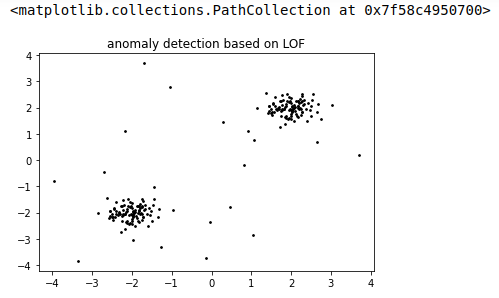
If you look into the data plot shown above, there are two major clusters (coming from datums_ variable), and then there are points in area with less density coming from our anomalies array.
Let’s prepare our LOF-based mode and run over data to see results:
Initiate mode for local outlier factor based anomaly detection.
clf = LocalOutlierFactor(n_neighbors=20, contamination=0.1)Here, the n_neighbors parameter determines the number of neighbors we consider to have processed to calculate the local outlier factor of each point. The contamination parameter is just a constant to determine the boundaries for inliers region and outliers region.
Lets call clf.fit_predcit() method to see which data points are outliers:
output=clf.fit_predict(dataset)
output
array([ 1, 1, 1, 1, 1, 1, 1, 1, 1, 1, 1, 1, 1, 1, 1, 1, 1,
1, 1, 1, 1, 1, 1, 1, 1, 1, 1, 1, 1, 1, 1, 1, 1, 1,
1, 1, 1, 1, 1, 1, 1, 1, 1, 1, 1, 1, 1, 1, 1, 1, 1,
1, 1, 1, 1, 1, 1, 1, 1, 1, 1, 1, 1, 1, 1, -1, 1, 1,
1, 1, 1, 1, 1, 1, 1, 1, 1, 1, 1, 1, 1, 1, 1, 1, 1,
1, 1, 1, 1, 1, 1, 1, 1, 1, 1, 1, 1, 1, 1, 1, 1, 1,
1, 1, 1, 1, 1, 1, 1, 1, 1, 1, 1, 1, 1, 1, 1, 1, 1,
1, 1, 1, 1, 1, 1, 1, 1, 1, 1, 1, 1, 1, 1, 1, 1, 1,
1, 1, 1, 1, 1, 1, 1, 1, 1, 1, 1, 1, 1, 1, 1, 1, 1,
1, 1, 1, 1, 1, 1, 1, 1, 1, 1, 1, 1, -1, 1, 1, 1, 1,
1, 1, 1, 1, 1, 1, 1, 1, 1, 1, 1, 1, 1, 1, 1, 1, 1,
1, 1, 1, 1, 1, 1, 1, 1, 1, 1, 1, 1, 1, -1, -1, -1, -1,
-1, -1, -1, -1, -1, -1, -1, -1, -1, -1, -1, -1, -1, -1, -1, -1])By looking into the array, we can see that points with less density coming from anomalies array have -1 score.
'''
get outliers scores
'''
datums_scores = clf.negative_outlier_factor_
'''
We will use this score to draw radius of each data point representing local outlier factor of that point
'''
Get radius array for data points according to scores.
radius = (datums_scores.max() - datums_scores) / (datums_scores.max() - datums_scores.min())
Plot the data set with LOF based radius of each datum.
plt.title('anomaly detection based on local outlier factor')
plt.scatter(dataset[:, 0], dataset[:, 1], color='k', s=3., label='datums')
plt.scatter(dataset[:, 0], dataset[:, 1], s=1000 * radius, edgecolors='r',
            facecolors='none', label='Outlier scores')
plt.axis('tight')
plt.xlim((-5, 5))
plt.ylim((-5, 5))
plt.show()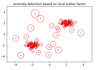
Here, first we drew datums, then circled around each datum coming from radius value based on LOF score of that datum. Now, based on the threshold we can mark any data point as normal datum or anomaly, maybe we can pick top 10 data points with largest circles and mark them anomalies.
So far we were working on a static dataset. In Part II of this tutorial, we will work on a time series dataset and see how anomalies behave when we are rolling down sliding window over time series dataset.
References
https://www.itl.nist.gov/div898/handbook/prc/section1/prc16.html
https://scikit-learn.org/stable/auto_examples/neighbors/plot_lof_outlier_detection.html
https://en.wikipedia.org/wiki/Outlier