Today, we are going to learn about Ordinary Least Squares Regression in statsmodels. Some of you may know that linear regression is a supervised machine learning model that determines the linear relationship between the dependent (y) and independent variables (x) by finding the best-fit linear line between them.
When there is only one independent variable and the model must find the linear relationship between it and the dependent variable, a simple linear regression is used.
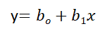
Here’s a Simple Linear Regression Equation, where bo denotes the intercept, b1 denotes the coefficient or slope, (x) denotes the independent variable, and (y) denotes the dependent variable.
The primary goal of a Linear Regression Model is to find the best fit linear line as well as the optimal intercept and coefficient values in order to minimize the error. The difference between the actual and predicted values is referred to as “error”, and the goal is to minimize it.
Assumptions of Linear Regression:
- Linearity: It states that the dependent variable (y) should be related to the independent variables linearly. A scatter plot between both variables can be used to test this assumption
- Normality: The (x) (independent) and (y) (dependent) variables should be normally distributed
- Homoscedasticity: For all values of (x), the variance of the error terms should be constant, i.e. the spread of residuals should be constant. A residual plot can be used to test this assumption
- Independence/No Multicollinearity: The variables must be independent of one another, with no correlation between the independent variables. A correlation matrix or VIF score can be used to test the assumption
- Error Terms: The error terms should be normally distributed. To examine the distribution of error terms, use Q-Q plots and Histograms. There should be no autocorrelation between the error terms. The Durbin Watson test can be used to determine autocorrelation. The null hypothesis is based on the assumption that there is no autocorrelation. The test’s value ranges from 0 to 4. If the test value is 2, there is no auto correlation
Let’s understand the methodology and build a simple linear regression using statsmodel:
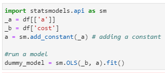
- We begin by defining the variables (x) and (y).
- The constant bo must then be added to the equation using the add constant() method
- To perform OLS regression, use the statsmodels.api module’s OLS() function. It yields an OLS object. The fit() method on this object is then called to fit the regression line to the data
- The summary() method is used to generate a table that contains a detailed description of the regression results from pandas import DataFrame
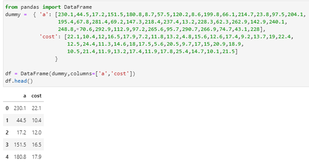
dummy = { ‘a’: [230.1,44.5,17.2,151.5,180.8,8.7,57.5,120.2,8.6,199.8,66.1,214.7,23.8,97.5,204.1,
195.4,67.8,281.4,69.2,147.3,218.4,237.4,13.2,228.3,62.3,262.9,142.9,240.1,
248.8,70.6,292.9,112.9,97.2,265.6,95.7,290.7,266.9,74.7,43.1,228],
‘cost’: [22.1,10.4,12,16.5,17.9,7.2,11.8,13.2,4.8,15.6,12.6,17.4,9.2,13.7,19,22.4,
12.5,24.4,11.3,14.6,18,17.5,5.6,20.5,9.7,17,15,20.9,18.9,
10.5,21.4,11.9,13.2,17.4,11.9,17.8,25.4,14.7,10.1,21.5]}
df = DataFrame(dummy,columns=[‘a’,’cost’])
df.head()
import statsmodels.api as sm
_a = df[[‘a’]]
_b = df[‘cost’]
a = sm.add_constant(_a) # adding a constant
#run a model
dummy_model = sm.OLS(_b, a).fit()
#predict
predict = dummy_model.predict(a)
print_model = dummy_model.summary()
print(print_model)
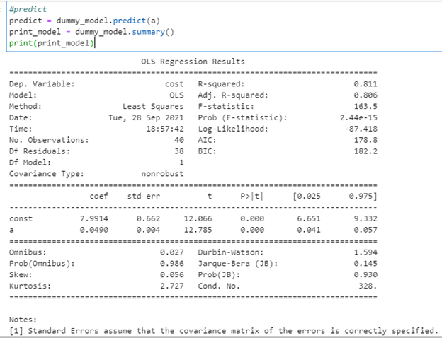
Let’s understand the summary report by dividing it into 4 sections:
SECTION 1:
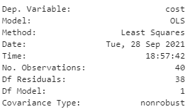
This section provides us with the basic details of the model that we can read and understand. Let’s take a look at: df (Residual) and df (Model Number). df is an abbreviation for “Degrees of Freedom”, which is the number of independent values that can vary in an analysis.
In regression, residuals are simply the error rate that is not explained by the model. It is the measurement of the distance between the data point and the regression line.
df(Residual) can be calculated as:
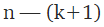
Where n is number of records, k is df(model).
SECTION 2:
R squared: The degree to which the dependent variables in (x) explain the variation in the dependent variable (y). In our case, we can say that 81.1% variance is explained by the model. The disadvantage of an R2 score is that as the number of variables in x increases, R2 tends to remain constant or even increase by a small amount. The new variable, on the other hand, may or may not be significant.
Adj. R square: This overcomes the disadvantage of the R2 score and is thus considered more reliable. Adj. R2 does not consider variables that are “not significant” for the model.
F statistic = Explained variance / unexplained variance.
The Fstat probability is lower than 0.05(alpha value). It means that the probability of getting 1 coefficient to be non zero is 2.44e-15.
Log-Likelihood: The maximum likelihood estimator is derived from the likelihood value, which is a measure of fit/goodness of model.
AIC and BIC: These 2 methods are used for scoring and selecting models.
SECTION 3:
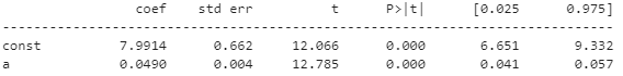
The column coef is the value b1.
Std err is the error of each variable (distance away from regression line)
T and P>|t| are the tstat values.
[0.025,0.975] – 5% alpha/95% confidence interval range, if coef value is in between this, it is called acceptance region.
SECTION 4:
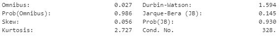
Omnibus: It determines whether the explained variance in a set of data is significantly greater than the unexplained variance in the aggregate. We hope that the Omnibus score is close to 0 and the probability is close to 1, indicating that the residuals follow normalcy.
Skew: It is a measure of data normalcy. It also drives omnibus and we the value of skew should be close to 0.
Kurtosis: Is a measure of curvature of data.
Durbin-Watson Test: Test is used to autocorrelation in the data.
JB and prob(JB): Is used to test the normality of data.
Cond no: Is used to check collinearity in the data.
Summary
To summarize, you can think of ordinary least squares regression as a strategy for obtaining a ‘straight line’ that is as close to your data points as possible from your model. Although OLS is not the only optimization strategy for this type of task, it is the most popular because the regression outputs (that is, coefficients) are unbiased estimators of the true values of alpha and beta.
References
- Official documentation for OLS
- Jupyter Book Online
- Analytics Vidhya