Data Courses

This article contains affiliate links. For more, please read the T&Cs.

Introduction

The decision tree is a machine learning algorithm which perform both classification and regression. It is also a supervised learning method which predicts the target variable by learning decision rules.

This article will demonstrate how the decision tree algorithm in Scikit Learn works with any data-set. You can use the decision tree algorithm with both classification and regression, which we will demonstrate separately. Plus, we’ll illustrate how you can visualize the decision tree created using Scikit-Learn decision tree model using GraphViz.

Decision Trees as Classification

Using Scikit Learn, you can apply the decision tree algorithm as a classification – DecisionTreeClassifier. We will use this classifier to demonstrate how it learns and predicts the outcome. For this purpose, we will use the Iris flower dataset available in Scikit Learn dataset library.

from sklearn.datasets import load_iris

As we are ready with the dataset, let’s now import the DecisionTreeClassifier model.

from sklearn.tree import DecisionTreeClassifier
 
iris = load_iris()
list(iris.keys())
['data', 'target', 'target_names', 'DESCR', 'feature_names', 'filename']

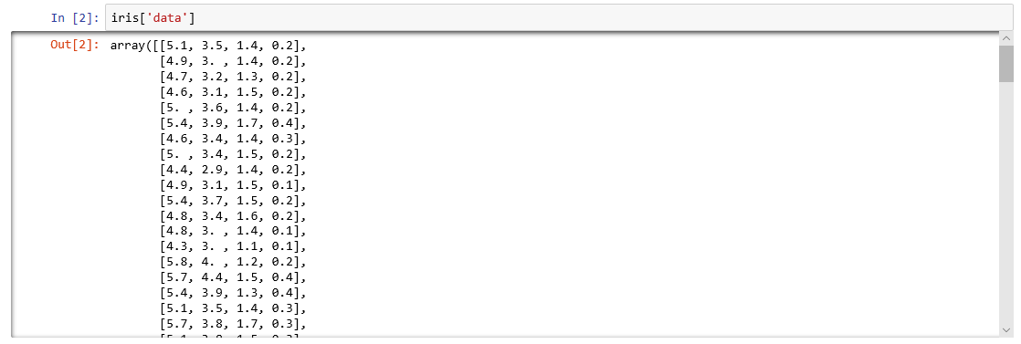
The Iris dataset consists of six columns, where we will consider only the first two columns for our demonstration – data & target. First, let’s load only the petal length and petal width, in a variable, for model training purpose. The data column is organized as sepal length, sepal width, petal length and petal width. We will consider only the third and fourth to obtain the petal length and petal width.

Second, let’s load the target column into another variable to label what type of iris flower are they – Iris Setosa, Iris Versicolor, and Iris Virginica.

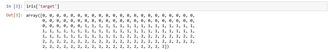
The zeroes represent Iris Setosa; the ones represent Iris Versicolor; and the two’s represent Iris Virginica.

X = iris.data[:, 2:] # The iris petal length & petal width
y = iris.target

Now it’s time to train the model with the dataset we have. We can use the fit() method to start training the model.

tree_clf = DecisionTreeClassifier(max_depth=2)
tree_clf.fit(X, y)

As the training is completed let’s test how the prediction works. Let’s input 3 dummy pair values – 5.6 & 2.4, 4.7 & 1.4, 1.3 & 0.2.

The values have returned 2, 1 and 0 which represents Iris Virginica, Iris Versicolor and Iris Setosa respectively. If you check this manually with our iris dataset, you can know that the predictions were accurate.

Visualizing Decision Tree – Classification

We can use the Graphviz module to visualize the classification decision tree model  predictions. The Scikit Learn’s export_graphviz module will export the visual in a dot format. So, you need Graphviz to convert it into a graphical format.

However, you need to install the Graphviz using pip install first.

pip install graphviz 

Note: You can also directly install graphviz from the official website. If you decide to install directly, make sure you create a new environmental variable path in your Windows device by adding the path of the bin file installation path. You can get the instructions of installing in the official website as well.

Now, let’s start to visualize our classification decision tree by importing the export_graphviz module which is available in Scikit Learn.

from sklearn.tree import export_graphviz

In order to avoid operating system issues, let’s use the image_path function that handles input and output operation. Make sure you provide the correct path where to output the dot file.

import os
 
def image_path(fig_id):
    if not os.path.isdir("DT"):
        os.mkdir("DT")
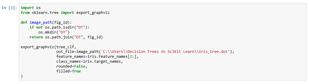
    return os.path.join("DT", fig_id)

Next, we will load tree_clf into the export_graphviz module so that it starts to visualize the decision tree.

export_graphviz(tree_clf,
                out_file=image_path('C:\\Users \\Decision Trees in SciKit Learn\\iris_tree.dot'),
                    feature_names=iris.feature_names[2:],
                class_names=iris.target_names,
                rounded=False,
                filled=True
)

You might wonder what iris.feature_names[2:] and iris.target_names does in this program. This is equivalent to [‘petal length (cm)’, ‘petal width (cm)’] and [‘setosa’, ‘versicolor’, ‘virginica’] respectively – just to get column names and classifications. The rounded attribute decides whether the edges should be round or not. The filled attribute decides whether each node needs a colour or not.

The above program will save a dot file in the path which is input. Let’s open this dot file using a notepad to see what exactly it contains.

Simply its a chunk of algorithm which we cannot understand. The idea behind the Graphviz is to convert this dot file in a graphical manner so that it will be easy to understand.

In order to do this, you will have to come out of the program. Open a command shell and type the following command. Make sure you change the directory to the location where the dot file is saved.

dot -Tpng iris_tree.dot -o iris_tree.png

This will convert the iris_tree.dot file into a png image format file and save it in the same location. 

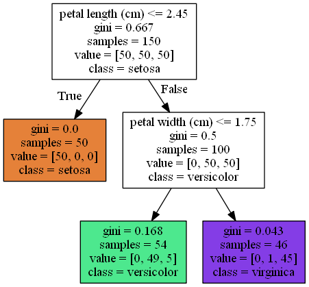
You will see a tree diagram visually like the above image displays. This will save in the same location as iris_tree.png file format.

When you want to classify an iris flower, you will start at the root node (depth 0). This node will ask if the petal length is less than or equal to 2.45 cm. If yes, it will move to the left node (depth 1) which is a leaf node. As it does not have any child node, it will predict the class which is Setosa.

Similarly, if the petal length is greater than 2.45 cm, it will move to the right node and ask whether the petal width is less than or equal to 1.75 cm. If yes, it will move to the left node (depth 2) and predict the class which is Versicolor, if not, it will move to the right node, and predict as Virginica.

The ‘samples’ attribute you see inside each node, is the number of times it applies the training instances. For example, the depth 1 left node has samples = 50, which means the petal length is less than or equal to 2.45 cm 50 times out of the total 150 samples.

The ‘value’ attribute you see inside each node, represents the number of occurrences of each class during the training. For example, depth 2 left node in green represents 0 times Setosa, 49 times Versicolor and 5 time Virginica occurrences.

The ‘gini’ attribute you see inside each node, represents the measure of impurity. If the value of gini is 0, you determine it as ‘pure’, where all the training data set belongs under the same class. For example, the depth 1 left node has gini=0 which means all the 50 samples belong to Setosa. 

However, the gini value is 1.168 and 0.043 respectively for other two classes. The equation used to calculate the gini value is shown below.

Here Pi,k is the ratio of class k instances among the training instances in the ith node.

Decision Trees as Regression

In Scikit Learn, the decision tree algorithm is available as a regression – DecisionTreeClassifier. We will use this regression model to demonstrate how it learns and predicts the outcome using the same dataset. First, Let’s import the regression model class.

from sklearn.tree import DecisionTreeRegressor

Now let’s load the data into the model and train it using the fit() method.

tree_reg = DecisionTreeRegressor(max_depth=2)
tree_reg.fit(X, y)

As we have completed the training process now, let’s see how the model prediction works. Let’s input the same 3 dummy pair values which we did in classification – 5.6 & 2.4, 4.7 & 1.4, 1.3 & 0.2.

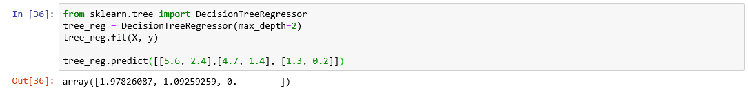
According to the output the regression model predicts the values as 1.97826087, 1.09259259 and 0.

Visualizing Decision Tree – Regression

We have discussed earlier about the Graphviz module and demonstrated the graphical representation for the decision-tree algorithm in classification. Now, we will follow the same process to visualize the regression decision tree.

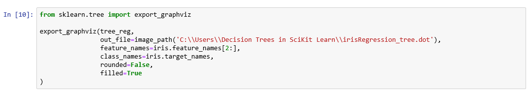
export_graphviz(tree_reg,
                    out_file=image_path(
           'C:\\Users\\ DecisionTreesinSciKit Learn\\irisRegression _ tree.dot '),
                    feature_names=iris.feature_names[2:],
                class_names=iris.target_names,
                rounded=False,
                filled=True
)

The only difference here is you must change the decision tree regression model (tree_reg), while others remain the same.

Now it will save the irisRegression_tree.dot file in the given path and we should convert it to a visual image using the command line.

dot -Tpng irisRegression_tree.dot -o irisRegression_tree.png

This will convert the irisRegression_tree.dot  file into a png image format file and save in the same location.

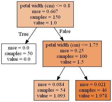
The tree diagram is the same as the classification, but here the output is not a class, but a value. The root node will ask you if the petal width is less than or equal to 0.8 cm.

If yes, it will traverse to the left node and output the value. However, If it is not the case, it will traverse to the right node and then ask if the petal width is less than or equal to 1.17 cm. If yes, the value will be 1.093, and if not, the value will be 1.978.

The prediction value is the average target value of the training instances within the leaf node and Mean Squared Error (MSE) is the results of all instances within the node. 

Conclusion

We hope this article gives you a clear idea of how you can utilize decision tree algorithm using Scikit Learn. We encourage you to apply this decision tree module with different datasets or even your own dataset. You can find all the other useful methods and functions of DecisionTreeClassifier and DecisionTreeRegressor from the official Scikit Learn documentation.  Additionally, there are examples of how decision trees and other classification techniques can be used in Chapter 9 of Mastering Maching Learning with scikit-learn.