Introduction

Logistic regression is an important model used in supervised learning. You can use logistic regression to estimate the probability of an instance which associates to a specific class. For example, with logistic regression, you can determine the probability of a new email is legit or spam. Likewise, you can also determine whether a student will pass or fail an exam, or a patient will have cancer or not and so on.

While you are reading this article, you may think about a dataset you have. See if you can train this model with that dataset and apply a logistic regression concept to predict a ‘yes class’ or ‘no class’ output. The reason we say either yes or no is because this model is dichotomous – only two decisions are output.

The logistic regression model predicts “positive” class if the probability of that instance is greater than 50% and labels it as “1”. On the other hand, if the probability of that instance is less than 50%, the model labels it as “0” and predicts “negative” class. In general, you can call logistic regression as a binary classifier.

Types of Logistic Regression

In the introduction, all we spoke is about binary logistic regression, where there are only two possible outcomes. However, applying some advanced techniques to logistic regression, you can determine Multinomial or Ordinal logistic regressions as well.

Multinomial logistic regression can have three or more nominal categories like predicting whether an animal is a cat, dog or cow. Ordinal logistic regression predicts three or more ordinal categories such as satisfaction rating between 1 to 5.

Understanding the Science behind Logistic Regression

The logistic regression model calculates the weighted sum for input features and outputs the logistic of the result. The logistic output is a sigmoid function that looks like the ‘S’ shaped curve in a graph which relies upon values between 0 and 1.

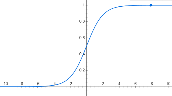
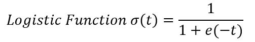
The above shown is the graph of how logistic function looks like and the equation of the logistic function. After the logistic regression model estimates the probability of an instance, then it can make predictions easily.

Working with Logistic Regression

SciKit Learn library is most famous among machine learning. SciKit Learn has the logistic regression model available as one of its features. We will use it to demonstrate today’s machine learning activity.

In our article today, we will use the dataset which has records of 150 Iris flowers. This famous dataset is common among data scientists to demonstrate machine learning concepts. The dataset contains details of sepal and petal length of iris flowers in three different species – Iris setosa, Iris versicolor, and Iris virginica.

Our goal is to build a model that determines whether the input value belongs to Iris Virginica species or not, relative to its petal width. Initially, to get started with the dataset, follow the below commands.

>>> from sklearn import datasets
>>> import numpy as npy
 
>>> iris = datasets.load_iris()
>>> list(iris.keys())
['data', 'target', 'target_names', 'DESCR', 'feature_names', 'filename']

Now we know all the information available in the dataset – data, target, target_names, DESCR, feature_names and filename. However, we will only play around with data & target.

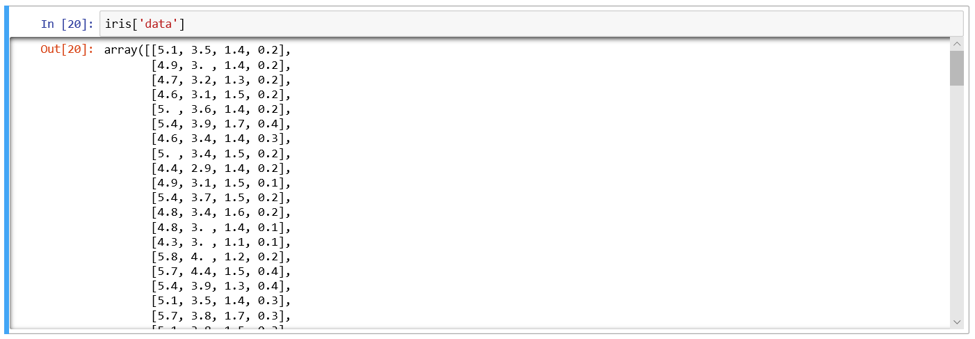
The data has information on sepal length and width, & petal length and width. We will assign all the petal width to the variable petalWidth.

>>> X = iris["data"][:, 3:] # width of the Petal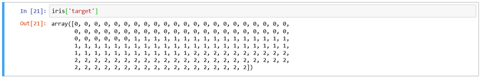

The target label 0 is for Iris-Setosa; label 1 is for Iris-Versicolor; label 2 is for Iris-Virginica. Therefore, we will assign label 2 in the variable label which specifies Iris-Virginica.

>>> y = (iris["target"] == 2).astype(npy.int) # Determine as 1 if Iris-Virginica, Else 0

Now let’s use this information to train our logistic regression model.

>>> from sklearn.linear_model import LogisticRegression
>>> logitRegression = LogisticRegression()
>>> logitRegression.fit(petalWidth, label)

As the training is complete, let’s evaluate the model by inputting sample petal width. Based on our input, the model will guess the probability of whether it might be Iris-Virginica or not. So, let us create 1000 sample data of petal width ranging between 0 to 3 in centimetres.

>>> X_new = npy.linspace(0, 3, 1000).reshape(-1, 1)

Now we can use the predict_proba() function to predict the outcome.

>>> y_proba = log_reg.predict_proba(X_new)

As the prediction is completed let us plot them in a graph to have a better understanding.

>>> import matplotlib.pyplot as plt
 
>>> plt.plot(X_new, y_proba[:, 1], "g-", label="Iris-Virginica")
>>> plt.plot(X_new, y_proba[:, 0], "b--", label="Not Iris-Virginica")
>>> plt.legend()
>>> plt.xlabel('Petal Width in cm')
>>> plt.ylabel('Probability')

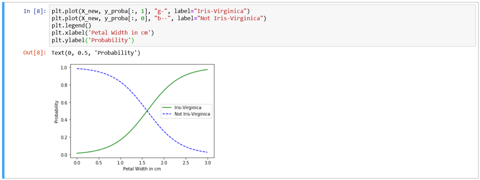
According to the visualization, the logistic regression model has confidence that petal width of more than 2 cm is Iris Virginica. On the other hand, below 1 cm petal width, the model is confident that it is not an Iris Virginica. In between 1 cm and 2 cm, the model is quite unsure.

We can also use the predict() function to see what the model thinks about individual petal lengths. Let’s input 1.5 cm to 1.8 cm width and get the output of its prediction.

>>> logitRegression.predict([[1.5],[1.6],[1.7],[1.8]])
array([0, 0, 1, 1])

According to the output, the model predicts Iris Virginica, only if the input width value is more than 1.6 cm. Furthermore, to examine the accuracy of the model prediction, you can evaluate the score given to this model. The score is examined by the score() function.

>>> score = logitRegression.score(X, y)
>>> score * 100, "%"
96.0 % 

As per the output, the model has an accuracy of 96%. Here accuracy means the number of correct predictions the model can predict, divided by the total number of predictions.

Advantages & Disadvantages of Logistic Regression

Logistic regression is an easy model to understand, interpret, implement and analyze. Many data scientists find this model convenient. However, logistic regression cannot handle a higher number of classes as it is vulnerable to model overfitting. 

Conclusion

This article educates you on how logistic regression helps to predict the probability of a class instance based on the training given to the model. You can extend this knowledge on the same dataset to find more information with other parameters. You can also apply this machine learning concept for your own dataset and see if you can improve the accuracy of the model. Finally, apply any dataset in real-world scenarios to obtain data-driven solutions and decisions.