This article contains affiliate links. For more, please read the T&Cs.
Importance of Merging & Joining Data
Many need to join data with Pandas, however there are several operations that are compatible with this functional action. Pandas provides many powerful data analysis functions including the ability to perform:
- Merging DataFrames
- Joining Data
- Appending
- Concatenation
These four areas of data manipulation are extremely powerful when used for fusing together Pandas DataFrame and Series objects in various configurations. All of these joins are in-memory operations very similar to the operations that can be performed in SQL.
Types of Joins
When we think about merging or joining data, we need to first remember the options available to us and what those options will ultimately mean for the output of our joining operation.
There are 6 distinct types of joins available to us, similar to those in SQL like statements:
- Left Join
- Full Outer Join
- Left Join (if NULL)
- Inner Join
- Right Join
- RIght Join (if NULL)

It is possible to join data with Pandas in each of these configurations as we’ll cover in the the below.
Example Data
In this tutorial, we make use of a dataset provided by FSU to fuse together data in various formats from the original dataset. If you’re following along in a Python script or a Jupyter Notebook you can access the data using the below functions.

file_name = "https://people.sc.fsu.edu/~jburkardt/data/csv/homes.csv"
df = pd.read_csv(file_name)
After loading the data into a DataFrame (df) we then clean up the column names to remove the extra ” and space values.
df.columns = ['Sell', 'List', 'Living', 'Rooms', 'Beds', 'Baths',
       'Age', 'Acres', 'Taxes']
Once this is performed we generate several additional DataFrames from our main DataFrame for usage down in our analysis of each of the merge, join, concat, and append functions. Those will be generated throughout this tutorial.
While working through this tutorial we’ll use several DataFrames to perform our joins: df; rooms; taxes; sb; & lb. The definitions for each are below, except for df which is defined earlier in our code:
rooms = df.groupby(['Rooms']).mean()
taxes = df[['Beds','Taxes']].groupby('Beds').mean().reset_index()
lb = df[df['large_beds']= True]
sb = df[df['large_beds'] == False]
merge() function in Pandas
The merge() function is one of the most powerful functions within the Pandas library for joining data in a variety of ways. There are large similarities between the merge function and the join functions you normally see in SQL. Its arguments are fairly straightforward once we understand the section above on Types of Joins.
merge contains nine arguments, only some of which are required values.
pd.merge(left, right, how='inner', on=None, left_on=None, right_on=None,
left_index=False, right_index=False, sort=True)
In the below, we generate an inner join between our df and taxes DataFrames. When this occurs, we’re selecting the on argument to be equal to the “Beds” column values. When this is done an additional column is created called “Taxes_y” which is the second column brought in from our taxes DataFrame. This column represents the average taxes per bedroom.
Inner Join
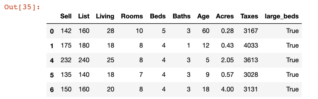
We can see from the below that the inner join actually did not remove any columns as each value from the inner join is present in the df DataFrame.
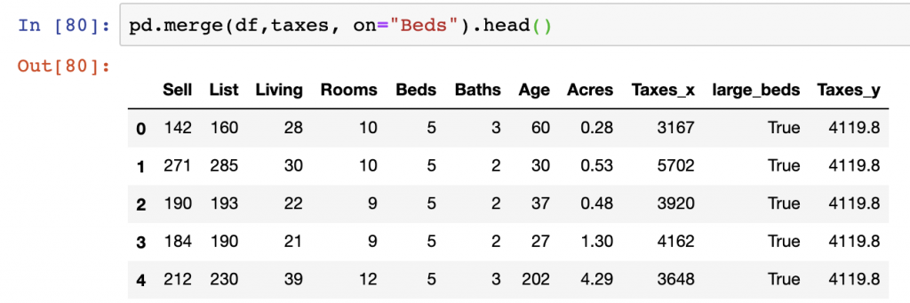
pd.merge(df,taxes, on="Beds").head()
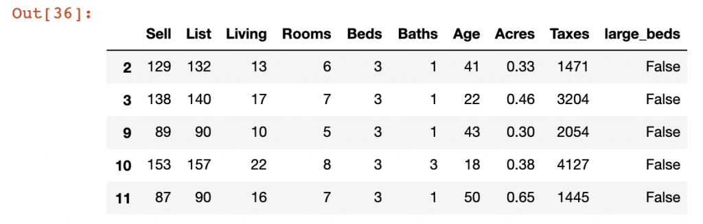
Left Join
The next type of join we’ll cover is a left join, which can be selected in the merge function using the how=”left” argument. We join the data from our DataFrames df and taxes on the Beds column and specify the how argument with ‘left’. The data is joined and adds a duplicative column named Taxes which gets represented as Taxes_x for the original value of Taxes per property in the dataset and Taxes_y for the average tax value per Bed number.
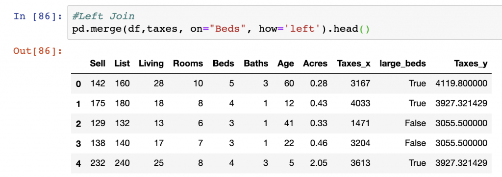
pd.merge(df,taxes, on="Beds", how='left')
Left Join (if NULL)
In this example, we’ll purposely join some data where there are missing values in the left DataFrame object that will result in some NaN values in our final or merged DataFrame output. We’ll use conditional logic to select specific rows in the taxes DataFrame and limit it by records where Beds is less than 4. We then join the main DataFrame df with the new taxes object.
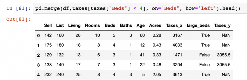
pd.merge(df,taxes[taxes["Beds"] < 4], on="Beds", how='left')
The result of the join shows that there are NaN records present as the new taxes DataFrame we used did not include records for Beds greater than 3.
We can clean up the names of the columns duplicated in the join by renaming the columns after the join operation is complete.
Right Join
Performing a right join is ultimately the reverse operation from a left join that we handled in the prior section. In the case of the right join, the right DataFrame specified will control which data remains present after the join is complete.
Here we use the df DataFrame as our left object in the merge() function and the augmented taxes DataFrame (from the above) on the right argument. We additionally specify the join to be on the “Beds” column using the on argument as well as specifying the type of join to be a “right” join in our how argument.
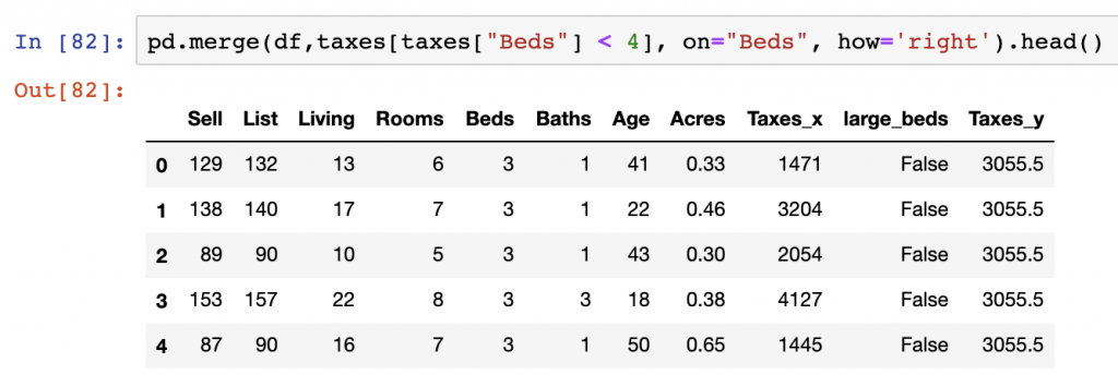
pd.merge(df,taxes[taxes["Beds"] < 4], on="Beds", how='right')
In the case of Right Join (if NULL), we don’t cover that currently in this tutorial as the logic is similar to the same operation using Left Join (if NULL).
Full Outer Join
A full outer join merges data on common (by default in the merge function) or specified columns from both sides of the join resulting in all data from both DataFrames being present at the end of the operation.
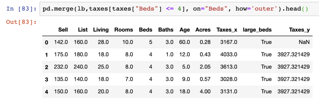
pd.merge(lb,taxes[taxes["Beds"] <= 4], on="Beds", how='outer')The resulting join in the above example shows that all of the taxes and large beds DataFrames are joined, however this produces some NaN values where there is not overlap between the two DataFrames on the specified join column, Beds. As our augmented taxes, DataFrame doesn’t include records for Beds equal to 5, we see that the first record contains a NaN Value under the Taxes_y column.

Multi-Column Joins
One of the similar features of the merge function to that of SQL logic is that joins can be specified across multiple columns. In the examples we’ve provided above, we haven’t shown this process, however it can be done using the on argument in the merge function.
A simple example of this is below where we will Left Join our data on the Beds and Baths columns between the df and taxes DataFrames. The reported values for avg_taxes will contain the average taxes for all Beds and Rooms combinations where data is present in the right DataFrame. All records remain in place for the df DataFrame.
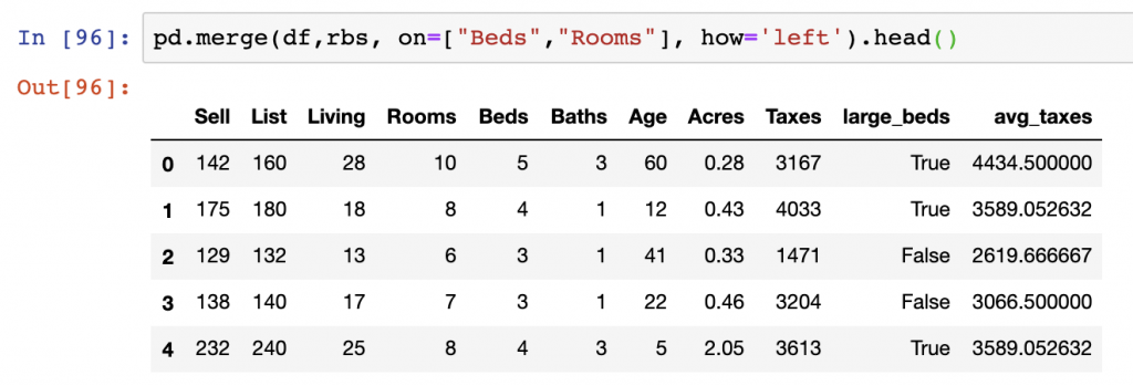
rbs = df.groupby(['Beds','Rooms'])['Taxes'].mean().reset_index()
rbs = rbs.rename(columns={"Taxes":"avg_taxes"})
pd.merge(df,rbs, on=["Beds","Rooms"], how='left')
join data with Pandas
While merge has to have a specification of the on argument to join two DataFrames together, join automatically will join DataFrames on their indices, however join also has arguments to perform LEFT, RIGHT, INNER, & FULL joins on either column names or indices. In this section, we will skip some of the join logic discussion as to not duplicate what was explained earlier in the merge section regarding how each type of join works.
The join function takes several arguments and is essentially used to perform joins based on the specification of the how argument and will join the DataFrame object with other – the secondary DataFrame or Series object.
DataFrame.join(self, other, on=None, how='left', lsuffix='', rsuffix='', sort=False)As stated, we don’t go into much detail on the logic of joins, but below are the examples of how to perform each type of the main join types:
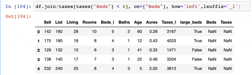
df.join(taxes[taxes["Beds"] < 4], on=["Beds"], how='left',lsuffix='_l')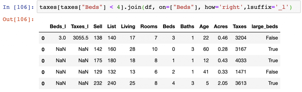
taxes[taxes["Beds"] < 4].join(df, on=["Beds"], how='right',lsuffix='_l')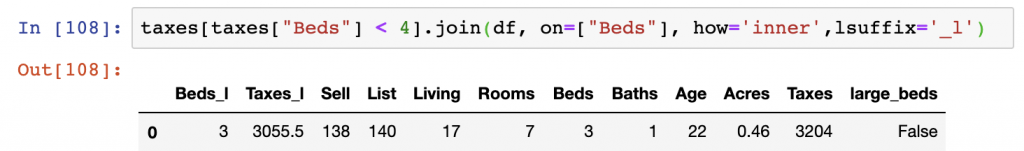
taxes[taxes["Beds"] < 4].join(df, on=["Beds"], how='inner',lsuffix='_l')This recap of the join and merge functions covers virtually all aspects of how to join data with Pandas. You should be able to, from this tutorial, manipulate DataFrames and Series by clasic SQL-like operations.
append()
The DataFrame.append() function is a simple operation of adding rows and columns to an existing DataFrame (or adding a Series records to an existing Series). In the land of comparison with SQL, the append and concat functions both serve purposes very similar to that of the UNION statement. This said Pandas helps manage some of the nuances of the UNION statement construction in SQL by imputing common column names from existing DataFrames to perform the append action.
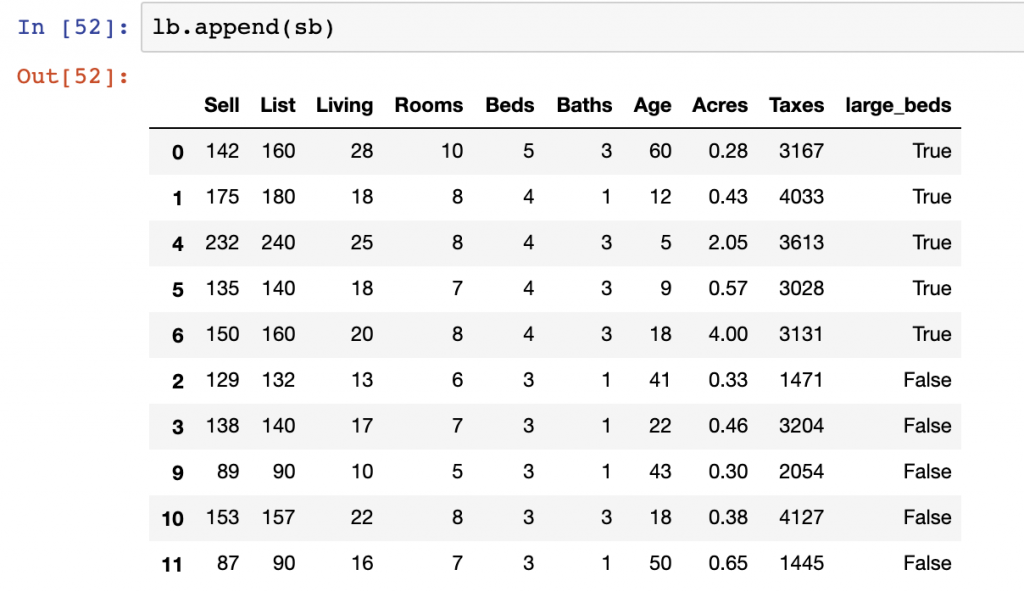
In our example, we have separated out records into a “Large Beds” and “Small Beds” DataFrames representing those records that have the number of Beds greater than 4 and those who fall below 4 respectively. We will use the append() function to add the Small Beds DataFrame to the Large Beds dataframe.


df['large_beds'] = df['Beds'] >= 4
lb = df[df['large_beds'] == True]
sb = df[df['large_beds'] == False]
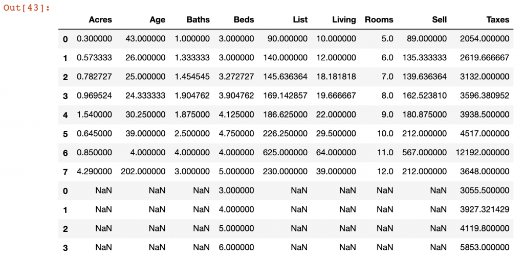
lb.append(sb)Note that you can use the append function in many different ways. For instance, we could append the Rooms and Taxes DataFrames together. Though this would likely be of limited analytical use, it provides an example of how the append function works. It ultimately finds commonly named columns and adds data to the existing DataFrame, even if those values are NaN. We see in this example below that the data from appending these two DataFrames together contains many NaN values and doesn’t provide excellent data quality.
append() has relatively few arguments to manage this operation, but the most useful of them is ignore_index which allows you reset the index you’re working with once the two files are appended to one another.
concat()
The concat function mirrors some of the examples we provided above with our explanation of append. It looks for common, however, it contains many additional arguments which make it more poweful than append. The example below mirrors what we have learned in the append function for illustrative purposes.
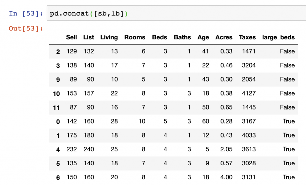
pd.concat([sb,lb])Looking a bit deeper into the concat function we see that it has more advanced features than append. Firstly, it can take in multiple DataFrames to perform its concatenation function. If we were to have multiple DataFrames to join, beyond simply two, we could do so by adding them together. An illustration of this would be the following:
pd.concat([sb,lb,taxes])In the above, all three DataFrames would be concatenated together in one single operation.
Summary
We’ve seen the power of merging, joining, concatenating, and appending data in this post. We learned the following critical points:
- Covered the 6 types of Join operations using merge and join
- Appended data using the append function
- Shown the power of the concat function
Now we know how to thoroughly manipulate DataFrames and Series objects using the approaches above. To expand our knowledge on merging, joining, and concatenating data, see the other examples from similar posts and resources:
- The Pandas official library documentation on merging, joining, & concatenating data
- Comparing merge/join functions in Pandas to SQL from the Pandas official documentation
- A longform post from Shane Lynn on their blog focused to merge and join data with Pandas
- Merging & Joining examples from Tutorials Point
- Pandas Merging, Joining, & Concatenating tutorial from Geeks for Geeks
- Chapter 7, “Data Wrangling: Clean, Transform, Merge, Reshape” in Python for Data Analysis
With this we should know exactly how to join data with Pandas, merge data with pandas, and concatenate data with Pandas.
The GitHub repo containing the code snippets for this content is here.