Data Courses

A Slimmed Down ETL

In this post, we provide a much simpler approach to running a very basic ETL. We will not be function-izing our code to run endlessly on a server, or setting it up to do anything more than – pull down data from the CitiBike data feed API, transform that data into a columnar DataFrame, and to write it to BigQuery and to a CSV file. Most of the details about the CitiBike feed from the prior post, we ignore here and assume you have some detail about them from our prior in-depth tutorials first section.

Setting Up Your Jupyter Notebook

First, make sure that you have the basic libraries below installed so that you can effectively write data to BigQuery. If you don’t or can’t you should skip the function on writing to BigQuery and will have to simply save the data into a CSV format.

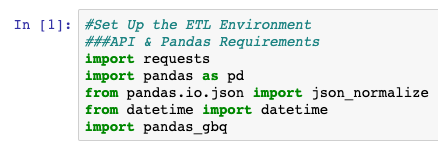
import requests
import pandas as pd
from pandas.io.json import json_normalize
from datetime import datetime
import pandas_gbq, pydata_google_auth #Requirements for Writing to BigQuery

For further details on how to set up your BigQuery environment, please see our prior post’s second section “Setting Up BigQuery“.

After confirming you have the prerequisites installed, boot up your Jupyter Notebook in the command line:

jupyter notebook

The next step is to, if you are following along the path of writing to BigQuery, list your connection and Google Project details for later use in the script:

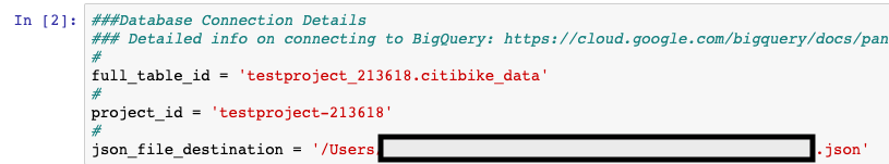
Your project details will differ from those above, but you will need to fill them out to connect and write to your BigQuery instance.

Your First API Call – Extracting the Data

Now that the basics of our Notebook are setup, we can start working on pulling data down with Requests. This is by far one of the simpler APIs to deal with on the internet and is provided by CitiBike’s station feeds. We chose it for specifically this reason as it is a great introduction to the Requests library and how it makes GET calls to API.

Here we simply assign our url variable with the feed URL and assign requests.get() to the variable r. Requests will be making a get call to that URL and extracting the currently available data.

url = "https://gbfs.citibikenyc.com/gbfs/en/station_information.json"
r = requests.get(url)

Transforming the Data

Now that we have our data saved into our r variable, we can begin extracting the important contents of the Stations feed. Here, we quickly access the .json structure of the data and stations level of the API response data and assign it to the stations variable.

stations = r.json()['data']['stations']

We want this data saved in this way as it is the data that is easily formatted to a columnar and DataFrame format.

Additionally, we want to extract data on the last time the CitiBike station updated the feed in order to understand the data if changes over time at some later date. Not only that, but we put the data into a human-readable format for storage purposes.

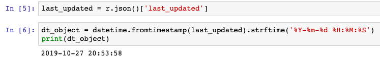
last_updated = r.json()['last_updated']

dt_object = datetime.fromtimestamp(last_updated).strftime('%Y-%m-%d %H:%M:%S')
print(dt_object)

The next step is to use the json_normalize function from Pandas and apply it to the .json object stored in the stations variable to load the data into a DataFrame. The next step is to generate and name a column called date to assign our last updated values to.

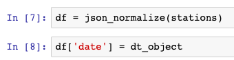
df = json_normalize(stations)
df['date'] = dt_object

Loading to the Database/CSV

Now that we have our data transformed from .json into a DataFrame we can then load the data into BigQuery using the simplistic to_gbq() function. There is one caveat here that if you’re doing this for the first time, you’re going to need to authorize your local laptop to write to your BigQuery project. This is mainly important for security purposes, so please follow the prompts you get in your Jupyter Notebook similar to the below.

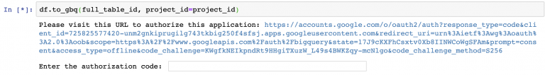
df.to_gbq(full_table_id, project_id=project_id)

Once the first data is written to BigQuery, you can go to it’s interface in your GCP Project and start querying your transformed data.

Alternatively, if you’re having trouble with the loading of data into BigQuery, you can write the data directly to a CSV file.

df.to_csv("citibike_stations_data.csv")

Is this still truly an ETL? You’re probably asking something similar. Yes, simply put we’ve Extracted, Transformed, and Loaded our data successfully.

For the code surfaced in the screenshots above, please visit our GitHub repository on Data Analysis. More information on common Pandas operations can be found in our detailed tutorials.