In this post, we’re going to show how to generate a rather simple ETL process from API data retrieved using Requests, its manipulation in Pandas, and the eventual write of that data into a database (BigQuery). The dataset we’ll be analyzing and importing is the real-time data feed from Citi Bike in NYC. The data is updated regularly (every few seconds) and can be accessed from the Citi Bike System Data feeds.
Once we have the data, several transformations will be applied to it to get it into a columnar format for insertion into our database. While we won’t cover in great detail getting setup with BigQuery for the first time, there are other tutorials which cover this setup in detail.
The Citi Bike Station Feed
Before we get started coding, we need to do what all analysis, engineers, and scientists must do before writing any code at all, understand the data. source. In this specific case, there are several data feeds we could potentially be interested in our construction of an ETL made available by Citi Bike’s endpoints.
The data we’re interested in is the real-time data provided by the GBFS system as is shown on the Citi Bike website below:

If you click on “Get the GBFS…” link you’ll be taken to a .json endpoint which has many other URL listed for sub-feeds in the system. We’re only interested in the first feed listed for our purposes which is highlighted:

If you put this link into your browser, you’re now able to see the lower level station information data available in the feed. The details of what exactly all of these feeds are is available on GitHub and is available in the below table:
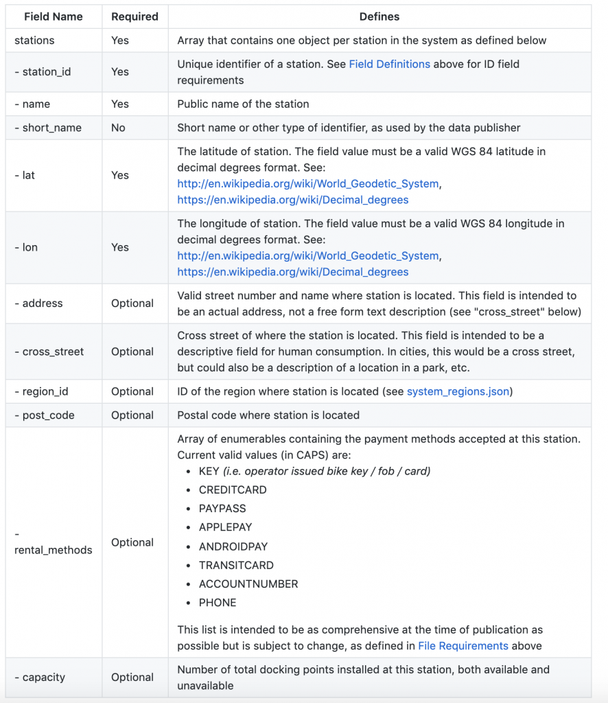
An example of a single row of data we’re looking to extract and store in BigQuery is below:
{"station_id":"237",
"external_id":"66db3c29-0aca-11e7-82f6-3863bb44ef7c",
"name":"E 11 St & 2 Ave",
"short_name":"5746.04",
"lat":40.73047309,
"lon":-73.98672378,"region_id":71,
"rental_methods":["CREDITCARD","KEY"],
"capacity":39,
"rental_url":"http://app.citibikenyc.com/S6Lr/IBV092JufD?station_id=237",
"electric_bike_surcharge_waiver":false,
"eightd_has_key_dispenser":false,
"eightd_station_services":
[{"id":"e73b6bfb-961f-432c-a61b-8e94c42a1fba",
"service_type":"ATTENDED_SERVICE",
"bikes_availability":"UNLIMITED",
"docks_availability":"NONE",
"name":"Valet Service",
"description":"Citi Bike Station Valet attendant service available","schedule_description":"",
"link_for_more_info":"https://www.citibikenyc.com/valet"}],
"has_kiosk":true}
Import Required Packages
Before we can import any packages we need to note a few things about the Python environment we’re using. Python 3 is being used in this script, however, it can be easily modified for Python 2 usage. This tutorial is using Anaconda for all underlying dependencies and environment set up in Python.
Now that we know the basics of our Python setup, we can review the packages imported in the below to understand how each will work in our ETL.
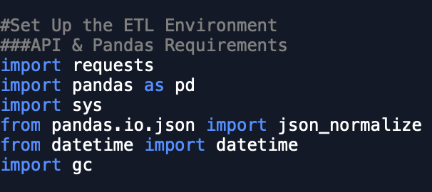
We first require Requests, which will be used to import our data from the .json feed into Python allowing for transformation using Pandas. You should notice however that we with Pandas, we actually import the entire library as well as the specific object json_normalize which is specifically designed to transform data from json objects into Dataframe objects.
Additional libraries that import are sys, datetime, and gc. sys is being used to call a system function that will help us stop Python from continuing in the case when certain criteria are met within our ETL. datetime is being used to transform datetime objects provided by the json API. Lastly, garbage collection, or gc is being used to clean up the memory footprint of our machine as we run our very basic ETL as a catch all to protect our laptop in case for some reason the script does not end as expected. All three of the above libraries are a part of the Python Standard Library.
Lastly, for connecting to BigQuery, we need to install pandas-gbq in our Python environment so that it is available for Pandas to use later in this post.
Setting Up BigQuery
Now that we understand the packages we’ll be using and Python is set up with everything we need to process the data, there is one last step before we can get started – enabling BigQuery. While this process seems straight forward, Google Cloud Platform is rapidly evolving and has changed several times since your author began using the platform several years ago. This said, here are the basics.
- Have a Google Account setup
- Set up a Google Cloud Platform Project
- Put in your credit card information for billing purposes
- Enable the BigQuery API in the GCP UI
- Authenticate your local client using a Jupyter Notebook or Python interpreter
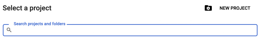
On step 2, we need to go to https://console.cloud.google.com/ and select in the upper left-hand side the “Create Project” icon. In the screenshot below we’ve already created a project called “testproject” which you will not see when you login for the first time. If you have an existing project you’d like to use, ignore this step.

Once you click on the dropdown to the right in the screenshot above, you’ll see the option to create a new Project. Once you click New Project and name your new project (with the default settings for this tutorial), we can continue on to enabling billing.
Step 3 requires your credit card information as BigQuery is ultimately a paid service. You’ll need to insert your billing details for your project in the GCP Billing console. Do not worry about cost at this point. BigQuery is notoriously cheap to use so much so that despite your author writing to BigQuery more than 5000 times in the current month and running many queries, their month to date cost of usage is a whopping $0.00. More details on BigQuery pricing can be found here.
For step 4, we need to go to this link and enable the BigQuery API. If BigQuery isn’t enabled, you’ll get errors trying to write data to the service, so don’t skip this step. More details on this can be found in the official documents.
Step 5 can be the most confusing area as there can be several ways to authenticate your client with CGP. The approach we’ll take is that of the one baked into the Pandas library using pandas-gbq. If you didn’t catch the installation step earlier in the tutorial, make sure you have pandas-gbq installed. We’ll cover the first time authentication to BigQuery later in this tutorial as it has a few prerequisites not yet covered.
Building API Ingestion Functions
Earlier we reviewed our data source and learned about it’s general structure. Now we need to import that data into Python successfully.
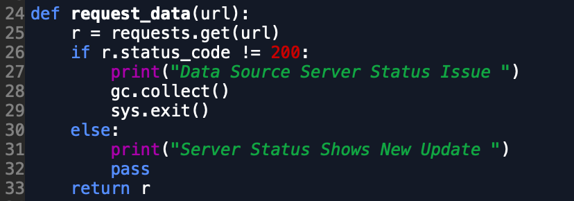
The Requests Library is commonly used to both get and request data through API. We’ll need to use the requests.get() function here to make a very simplistic pull from the endpoint we reviewed earlier. Firstly, we need to have a URL to pull the data from, which is shown hard-coded into the screenshot of our code below. Don’t worry so much about the other variables at this time. The only one important to us here is url.
Inserting url into the requests.get() function should return a requests object for us that contains the contents of our API feed from Citi Bike as well as some information about the API call itself. As we set our requests function response equal to r, we should check if the r.status_code variable is 200. If it is not, something is either wrong with our url variable or wrong with the API service itself as this endpoint should be open and accessible to the world.
In the code below, we can see that checking if the response is equal to 200 is a critical checkpoint in our ETL to ensure the response was worthy of continuing our code or not. If the response is not 200, we want to use sys.exit() to ensure the script doesn’t continue running when executed.
The other step we should take when we set the value of r is to look at r.json() to confirm that there is a json object assigned to that variable similar to the sample data above in our second section. If there is, we’re ready to move onto the next section.
Transforming Data in a DataFrame
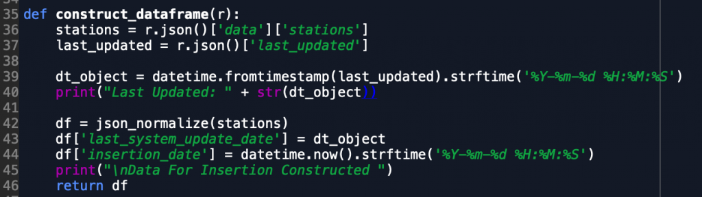
Earlier we walked through some of the aspects of the code within our request_data() function that requests the json feed from the Citi Bike endpoint. Now that we have successfully received that data and it is assigned to our variable r, we want to transform it into a format that suits BigQuery and our querying needs. For this we’ll need json_normalize. This function helps take json data and puts it into a columnar DataFrame format in Pandas. This makes our ETL efforts more streamlined as we can then put the data into an easier to access format than its original json format.
In our transformation steps below we access the json object in r and access the data and stations list that contains the real-time station by station data. Once we set that value to stations, as shown below, we want to also assign a variable equal to the json object last_updated which tells us the last time the station data was updated by the Citi Bike system. This is an important variable as in our next tutorial we will cover how to run this script over and over again to store data endlessly, however we don’t want to store duplicative records from the same system update time as that would make our end analysis less useful. We then quickly update the last updated object from a timestamp object to a human-readable object using the datetime library.
Now that that is complete, we are ready to initialize our DataFrame variable with the normalized stations json object. This is done quickly and we can then assign a column of the dataframe equal to our last_update variable so we know which time the rows correspond to.
At this point our DataFrame object set to the df variable should be fully ready for insertion into BigQuery. While there are some details that we skipped over from the function above, those will be picked up in our next part of this tutorial.
Writing Data to a Database
We mentioned earlier in the 5th step of getting BigQuery setup that we would have to circle back to authenticating your local environment for the first time and will do so now.
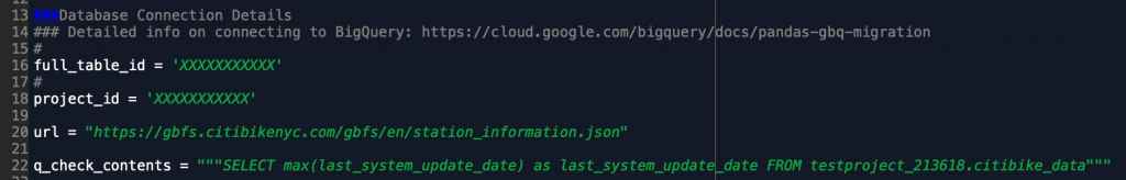
Earlier we created a GCP Project and that project comes with an ID. This ID needs to be entered to the project_id variable as seen below. Additionally, in the BigQuery UI we can choose to generate a table name for use in this ETL. Once we run our insertion script for the first time, the table will be automatically generated for us. Fill out the table name you want to name your project in the full_table_id variable.

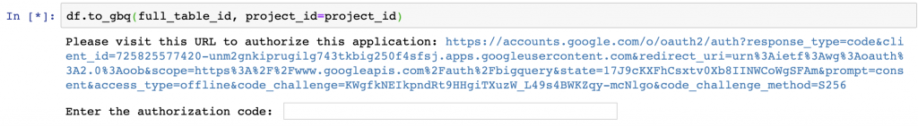
Now we need to manually authenticate to the GCP Project for the first time by executing the DataFrame.to_gbq() function with our full_table_id and project_id. When we execute this function we should be prompted something similar to the below by Google’s endpoints to provide an authentication code. Use the URL provided to copy and paste the authentication code from the Google Account you set up your GCP Project under. Once this is entered, you will be able to proceed to insert data into your BigQuery table.
One other consideration to take into account when inserting data into BigQuery is what is known as Chunking. In the example here, we only need to insert several hundred rows of data at a time, which BigQuery easily handles and will not drastically impact your network. When you have substantially larger DataFrame objects to insert into your database, you can call the chunksize argument in to_gbq() to insert only a given amount of records at a time, say 10k at a time. This will help your load of data into BigQuery without a traffic jam occurring in your data loads.
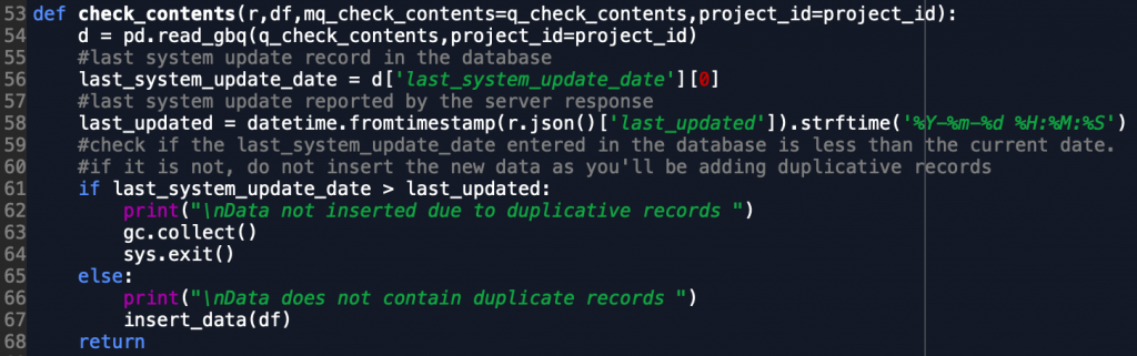
Building Data Quality Tests
One last step we perform in the ETL is to ensure that on runs of the ETL we don’t have duplicative records entered into the database. This can often happen with basic runs of an ETL due to several upstream reasons in our API data. In this case, we constantly check to see whether the system update date in the database is less than the last date pulled from the API. This helps prevent us having duplicative records by only allowing new data to flow through the ETL if there is for some reason a slow-down in the upstream Citi Bike API.