A “Statsmodels Module” is used to run statistical tests, explore data and estimate different statistical models. The Python Statsmodels Library is one of the many computational pillars of Python geared for statistics, data processing and data science. It is built on SciPy (pronounced “Sigh Pie”), Matplotlib, and NumPy, but it includes more sophisticated statistical testing and modeling functions not found in SciPy or NumPy.
This method for statistical analysis is more aligned with R, making it easier to use for those who are already familiar with R and want to move to Python.
Why Statsmodels?
statsmodels is built for hardcore statistics. The core of the Statsmodels Library is “production ready”. Traditional models like robust linear models, generalized linear model (GLM) etc. have all been around for a long time and have been validated against “R & Stata”. It also contains the time series analysis section, which includes vector autoregression (VAR), AR & ARMA.
Some Features Of Statsmodels
- Linear/ Multiple regression – Linear regression is a statistical method for modeling the linear relationship between a dependent variable and one or more explanatory variables. When there is only one independent/explanatory variable, it’s called “Simple Linear Regression”. “Multiple Linear Regression” is used in the case of multiple independent variables
- Logistic regression – The logistic model is used in statistics to model the likelihood of a specific event/class occurring such as win/lose, pass/fail, etc. This can be extended to model a variety of events
- Time series analysis – It refers to the analysis of time series data to retrieve meaningful statistics and many other data characteristics
- Statistical tests – Refers to the many statistical tests that can be done using the Statsmodels Library. Have a look at the official documentation
Difference Between Statsmodels OLS And Scikit Linear Regression
In statsmodels, you can get the prediction in the same way as scikit-learn, with the exception that we use the results instance returned by fit.
predictions = results.predict(X_test)
We can measure statistics based on the prediction error.
prediction_error = y_test – predictions
There is a different list of functions for calculating goodness of fit of prediction statistics, but it’s not incorporated into the models, and it doesn’t include R squared. Calculating these take a little more effort for the user, and statsmodels does not have the same collection of statistics, especially not for classification /models with a binary answer variable.
In its simple form, linear regression is the same in statsmodels and scikit-learn. The implementations, however, vary, which can result in different outcomes in edge cases, and scikit-learn supports larger models in general. Sparse matrices, for example, are used in only a few sections of statsmodels.
statsmodels essentially follows the standard model, in which we want to know how well a given model suits the results, what variables “describe” or “affect” the result, and the magnitude of the effect. Scikit-learn follows the machine learning pattern of selecting the “best” model for prediction as the key supported mission.
So, the stress in statsmodels supporting features is on training data analysis, and it means using hypothesis tests and goodness-of-fit steps. On the other hand, the focus in scikit-supporting learn’s infrastructure is on model selection for out-of-sample forecast, and thus cross-validation on “test data.”
In a time series problem, statsmodels also performs prediction and forecasting. When doing cross-validation for prediction in statsmodels, however, it is still always easier to use scikit-cross-validation learn’s setup in conjunction with statsmodels’ estimation models. Now, to continue with our tutorial on what is Python statsmodels library.
Linear Regression In Python Using Statsmodels
Linear regression, as previously explained, is a model that assumes a linear relationship between the dependent variable and the independent/exploratory variable(s).
Only one input variable is used to estimate the dependent variable in linear regression. Its equation is as follows:
y = ax +b
- y = Dependent variable (output)
- a = Slope of the regression line (the effect that x has on y)
- c = Constant (y Intercept)
- x = Independent variable (input variable used in predicting y)
For Multiple Linear Regression, the equation is (multiple independent variables):
y = b + a1x1 + a2x2+ …..+anxn
An Example
Let us create a dummy data set for stocks in New York Stock Exchange as shown:
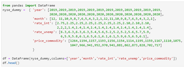
from pandas import DataFrame
nyse_dummy = { ‘year’: [2019,2019,2019,2019,2019,2019,2019,2019,2019,2019,2019,2019,
2020,2020,2020,2020,2020,2020,2020,2020,2020,2020,2020,2020],
‘month’: [12, 11,10,9,8,7,6,5,4,3,2,1,12,11,10,9,8,7,6,5,4,3,2,1],
‘rate_int’: [2.75,2.25,2.25,2.25,2.25,2.25,2.25,2.10,2.10,2.10,
2,2,2,1.4,1.4,1.4,1.4,1.4,1.4,1.4,1.4,1.4,1.4,1.4],
‘rate_unemp’: [6.3,6.3,6.3,6.3,5.4,5.6,5.2,5.2,5.2,5.6,5.7,5.9,
6,5.9,5.8,6.1,6.5,6.1,6.1,6.1,5.9,6.5,6.5,6.1],
‘price_commodity’: [1264,1194,1157,1193,1156,1154,1114,1195,1159,1167,1110,1075,
1047,966,941,952,970,941,881,862,873,828,702,717]
}
df = DataFrame(nyse_dummy,columns=[‘year’,’month’,’rate_int’,’rate_unemp’,’price_commodity’])
df.head()
Simple Linear Regression is shown in the Python code below, with the following input variables:
- Rate of Interest
This variable is being used to estimate the NYSE price commodity which is the dependent variable.
Here’s how we can do linear regression in Python with statsmodels:
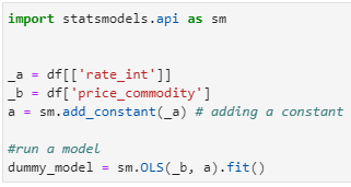
import statsmodels.api as sm
_a = df[[‘rate_int’]]
_b = df[‘price_commodity’]
a = sm.add_constant(_a) # adding a constant
dummy_model = sm.OLS(_b, a).fit()
Then, run the below code to check performance of the model:
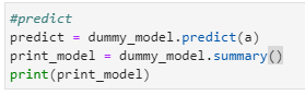
#predict
predict = dummy_model.predict(a)
print_model = dummy_model.summary()
print(print_model)
This result is displayed once you execute the code:
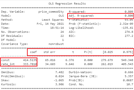
Let us interpret the results one by one:
- Adjusted R squared measures how well the model fits the data. The range of R squared values is 0 to 1, with a higher value indicating better fit
- The Y-intercept is the constant coefficient
- The change in the output Y due to a one-unit change in rate of interest is represented by the Interest Rate Coefficient (everything else being constant)
- Statistical significance is defined as a p-value of less than 0.05. When P is equal or less than 0.05, it means there is a lot of evidence to refute the null hypothesis
- The standard error of the coefficients is expressed by std err. Lower the values means higher accuracy
Let us predict the stock price as per our model results:
Recall the equation:
y = ax +b
…which in our terms, means:
price_commodity = (rate_int coeff) * X + const coeff
Let us take values for last month in 2019:
Rate_int in Dec’19 = 2.75
price_commodity = (333.78)*2.75 + 414.51 = 1332.40
Actual price of commodity in Dec’19 = 1264
Our prediction is off by = 1264 – 1332.40 = -68.4
Let us include another variable rate_unemp to predict stock price and see if our model improves:
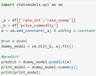
import statsmodels.api as sm
_a = df[[‘rate_int’,’rate_unemp’]]
_b = df[‘price_commodity’]
a = sm.add_constant(_a) # adding a constant
#run a model
dummy_model = sm.OLS(_b, a).fit()
#predict
predict = dummy_model.predict(a)
print_model = dummy_model.summary()
print(print_model)
Result:
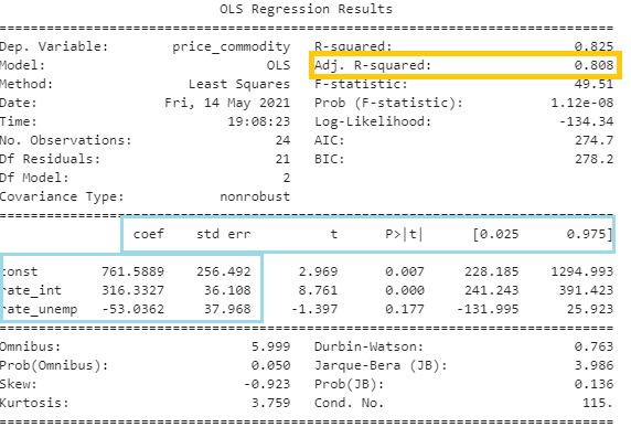
Let’s again calculate the commodity price for Dec ’19:
price_commodity = (rate_int coeff) * X1 +(rate_unemp)*X2 + const coeff
Let us take values for last month in 2019:
Rate_int in Dec’19 = 2.75
price_commodity = (316.33)*2.75 + (-53.03)*6.3 + 761.58= 1297.4
Actual price of commodity in Dec’19 = 1264
Our prediction is off by = 1264 – 1297.4 = -33.39
The model has improved slightly with the introduction of one more variable as we can notice that in the prediction and adjusted R squared value.
What do you think will happen when you will add year and month to the equation? Try it out!
(Note: This is fictional data created for practice purposes.)
Summary
statsmodels is based on SciPy, Matplotlib and NumPy. It includes advanced statistical testing functions, and comes with a plethora of descriptive statistics, statistical tests, result statistics and plotting functions. Matplotlib Library is used to power its graphical functions.
References
- Official documentation for statsmodels library
- Different use cases of statsmodels library
- Jupyter Book Online
- Wikipedia