In the previous chapter, we used a straight line to describe the relationship between the predictor and the response in Ordinary Least Squares Regression with a single variable. Today, in multiple linear regression in statsmodels, we expand this concept by fitting our (p) predictors to a (p)-dimensional hyperplane.
Multiple Linear Regression Equation:
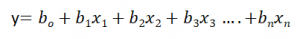
Let’s understand the equation:
- y – dependent variable
- b0 – refers to the point on the Y-axis where the Simple Linear Regression Line crosses it
- b1x1 – regression coefficient (b1) of the first independent variable (X1)
- b2x2 – regression coefficient of the last independent variable.
Let’s Understand Multiple Regression With Simple Example
Let’s say you’re trying to figure out how much an automobile will sell for. The selling price is the dependent variable. Imagine knowing enough about the car to make an educated guess about the selling price. These are the different factors that could affect the price of the automobile:
- Distance covered
- Power of the engine
- Automobile condition
- Year of production
Here, we have four independent variables that could help us to find the cost of the automobile.
Assumptions Of Multiple Linear Regression
Simple linear regression and multiple linear regression in statsmodels have similar assumptions. They are as follows:
- Errors are normally distributed
- Variance for error term is constant
- No correlation between independent variables
- No relationship between variables and error terms
- No autocorrelation between the error terms
Modeling With Python
Now, we’ll use a sample data set to create a Multiple Linear Regression Model.
Let’s take the advertising dataset from Kaggle for this.
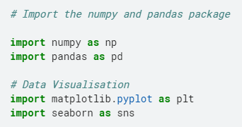
- Let’s import libraries that we need:
# Import the numpy and pandas package
import numpy as np
import pandas as pd
# Data Visualisation
import matplotlib.pyplot as plt
import seaborn as sns
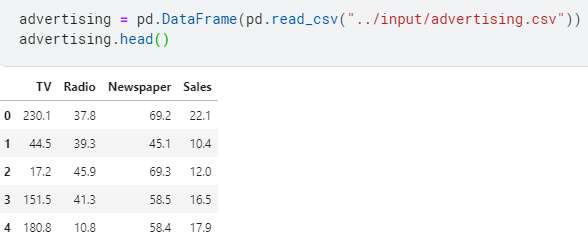
- Let’s load the dataset:
advertising = pd.DataFrame(pd.read_csv(“../input/advertising.csv”))
advertising.head()
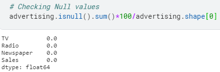
- Check null values:
advertising.isnull().sum()*100/advertising.shape[0]
- Check for outliers:
fig, axs = plt.subplots(3, figsize = (5,5))
plt1 = sns.boxplot(advertising[‘TV’], ax = axs[0])
plt2 = sns.boxplot(advertising[‘Newspaper’], ax = axs[1])
plt3 = sns.boxplot(advertising[‘Radio’], ax = axs[2])
plt.tight_layout()
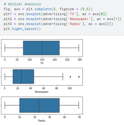
There are no considerable outliers in the data.
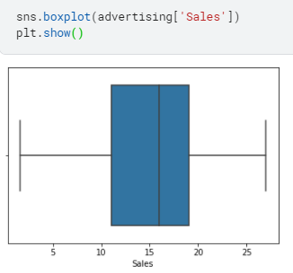
- Univariate and bivariate analysis:
sns.boxplot(advertising[‘Sales’])
plt.show()
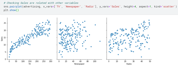
# Checking sales are related with other variables
sns.pairplot(advertising, x_vars=[‘TV’, ‘Newspaper’, ‘Radio’], y_vars=’Sales’, height=4, aspect=1, kind=’scatter’)
plt.show()
- Let’s check the correlation:
sns.heatmap(advertising.corr(), cmap=”YlGnBu”, annot = True)
plt.show()
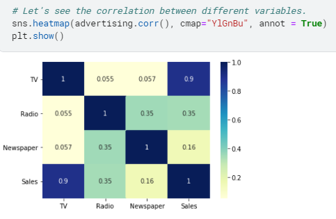
There’s no correlation in the data.
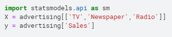
- Let’s build the model
import statsmodels.api as sm
X = advertising[[‘TV’,’Newspaper’,’Radio’]]
y = advertising[‘Sales’]
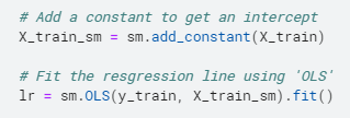
# Add a constant to get an intercept
X_train_sm = sm.add_constant(X_train)
# Fit the resgression line using ‘OLS’
lr = sm.OLS(y_train, X_train_sm).fit()
print(lr.summary())
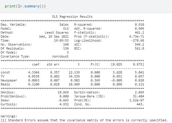
Understanding the results:
- Rsq value is 91% which is good. It means that the degree of variance in Y variable is explained by X variables
- Adj Rsq value is also good although it penalizes predictors more than Rsq
- After looking at the p values we can see that ‘newspaper’ is not a significant X variable since p value is greater than 0.05
- The coef values are good as they fall in 5% and 95%, except for the newspaper variable.
Summary
Our models passed all the validation tests. Thus, it is clear that by utilizing the 3 independent variables, our model can accurately forecast sales. However, our model only has an R2 value of 91%, implying that there are approximately 9% unknown factors influencing our pie sales.
References
- Official documentation for OLS
- Jupyter Book Online