What is Regression?
In the simplest terms, regression is the method of finding relationships between different phenomena. It is a statistical technique which is now widely being used in various areas of machine learning. In this article, we are going to discuss what Linear Regression in Python is and how to perform it using the Statsmodels python library.
In today’s world, Regression can be applied to a number of areas, such as business, agriculture, medical sciences, and many others. Regression can be applied in agriculture to find out how rainfall affects crop yields. In medical sciences, it can be used to determine how cognitive functions change with aging.
When it comes to business, regression can be used for both forecasting and optimization. So you can use it to determine the factors that influence, say productivity of employees and then use this as a template to predict how changes in these factors are going to bring changes in productivity. This can help you focus on factors that matter the most so that you can optimize them and bring about an increase in the overall productivity of employees.
An Example of Regression
When performing regression analysis, you are essentially trying to determine the impact of an independent variable on a dependent variable.
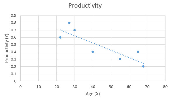
Let’s take our productivity problem as an example. We know that productivity of an employee is dependent on other factors. So productivity is the dependent variable. It may be dependent on factors such as age, work-life balance, hours worked, etc. These are the independent variables.
If X is one of these independent variables and Y, the dependent variable, then it would be possible to plot observed data of age and productivity into a scatter chart. What regression then does is model the relationship between these two variables by fitting an equation to the data distribution.
What is Linear Regression?
Linear regression is the simplest of regression analysis methods. When you plot your data observations on the x- and y- axis of a chart, you might observe that though the points don’t exactly follow a straight line, they do have a somewhat linear pattern to them. This is when linear regression comes in handy. It determines the linear function or the straight line that best represents your data’s distribution. As such, linear regression is often called the ‘line of best fit’.
Simple Linear Regression
When you have to find the relationship between just two variables (one dependent and one independent), then simple linear regression is used. The independent variable is usually denoted as X, while the dependent variable is denoted as Y.
Simple linear equation consists of finding the line with the equation:
Y = M*X +C
where,
M is the effect that X (the independent variable) has on Y (the dependent variable). In other words, it represents the change in Y due to a unit change in X (if everything else is constant).
C is called the Y-intercept or constant coefficient. This means, if X is zero, then the expected output Y would be equal to C.
A Diagrammatic Representation of Simple Linear Regression
The following diagram can give a better explanation of simple linear regression. Consider the following scatter diagram of variables X against Y. The blue dots are the actual observed values of Y for different values of X.
Let the dotted line be the regression line that has been calculated by regression analysis. This line can be represented as:
Y = M*X +C
Here, M is the slope of the dotted line.
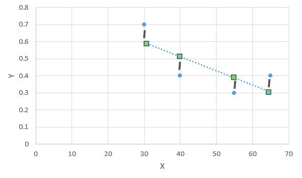
If you take any point on this line (green square) and measure its distance from the actual observation (blue dot), this will give you the residual for that data point. The sum of squares of all the residuals (SSR) can give you a good idea about how close your line of regression is to the actual distribution of data.
So, in regression analysis, we are basically trying to determine the dotted line that best minimizes the SSR. This approach of regression analysis is called the method of Ordinary Least Squares.
Multiple Linear Regression
In real circumstances very rarely do phenomena depend on just one factor. You will find that most of the time, the dependent variable is dependent on more than one independent variables. When linear regression is applied on a distribution with more than one independent variables, it is called Multiple Linear Regression.
Multiple Linear Regression consists of finding a plane with the equation:
Y = C + M1*X1 + M2*X2 + …
where,
- X1, X2, X3, etc. are independent variables
- M1, M2, M3, etc. are coefficients corresponding to X1, X2, X3, etc.
- C is called the constant coefficient.
When performing multiple regression analysis, the goal is to find the values of C and M1, M2, M3, … that bring the corresponding regression plane as close to the actual distribution as possible.
Using Statsmodels to perform Simple Linear Regression in Python
Now that we have a basic idea of regression and most of the related terminology, let’s do some real regression analysis.
We will perform the analysis on an open-source dataset from the FSU. This dataset contains data on the selling price, list price, living space, number of bedrooms, bathrooms, age, acreage and taxes. We will be using Jupyter Notebooks as our coding environment.
To begin with, let’s import the dataset into the Jupyter Notebook environment.
- Import necessary packages/ libraries: (Pandas)
import pandas as pd
from pandas import DataFrame- Read the CSV file from the URL location into a pandas dataframe:
myurl='https://people.sc.fsu.edu/~jburkardt/data/csv/homes.csv'
df = pd.read_csv(myurl)- Modify the header line to ensure we get the names in the format that we want.
df.columns = ['Sell', 'List', 'Living', 'Rooms', 'Beds', 'Baths', 'Age', 'Acres', 'Taxes']- Check the first few rows of the dataframe to see if everything’s fine:
df.head()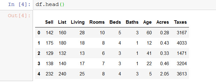
Let’s first perform a Simple Linear Regression analysis. We will use the Statsmodels python library for this.
Why Use Statsmodels and not Scikit-learn?
When performing linear regression in Python, it is also possible to use the sci-kit learn library. However, we recommend using Statsmodels. This is because the Statsmodels library has more advanced statistical tools as compared to sci-kit learn. Moreover, it’s regression analysis tools can give more detailed results.
- Let’s get all the packages ready. Make sure you have numpy and statsmodels installed in your notebook. If you don’t, you can use the pip install command to download and install both packages. After that, import numpy and statsmodels:
import numpy as np
import statsmodels.api as sm- Among the variables in our dataset, we can see that the selling price is the dependent variable. Let’s assign this to the variable Y. For simple linear regression, we can have just one independent variable.
So let’s just see how dependent the Selling price of a house is on Taxes. Let’s assign ‘Taxes’ to the variable X.
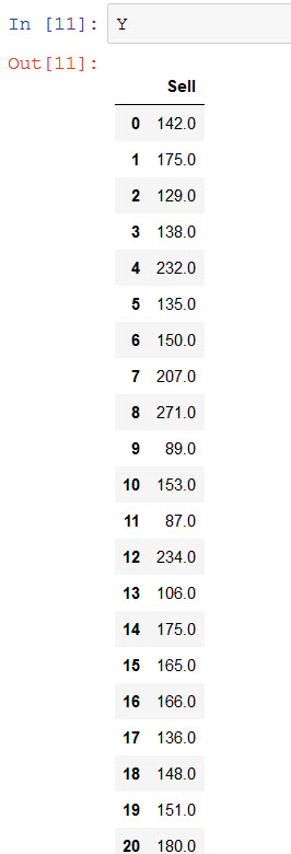
X = df[['Taxes']]
Y = df[['Sell']]
We will use the OLS (Ordinary Least Squares) model to perform regression analysis. This is available as an instance of the statsmodels.regression.linear_model.OLS class. Note that Taxes and Sell are both of type int64.But to perform a regression operation, we need it to be of type float.
- We can simply convert these two columns to floating point as follows:
X=X.astype(float)
Y=Y.astype(float)- Create an OLS model named ‘model’ and assign to it the variables X and Y. Once created, you can apply the fit() function to find the ideal regression line that fits the distribution of X and Y.
Both these tasks can be accomplished in one line of code:
model = sm.OLS(Y,X).fit()The variable model now holds the detailed information about our fitted regression model.
- To take a look at these details, you can summon the summary() function and print it as follows:
print(model.summary())Understanding the Results
Let us look at this summary in a little detail. We have highlighted the important information in the screenshot below:
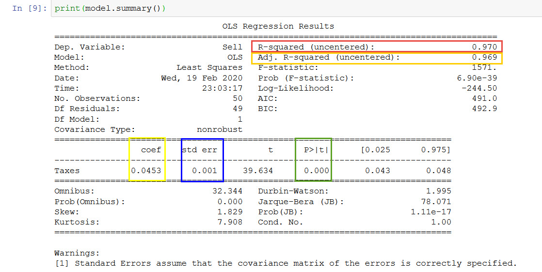
R-squared value: This is a statistical measure of how well the regression line fits with the real data points. The higher the value, the better the fit.
Adj, R-squared: This is the corrected R-squared value according to the number of input features. Ideally, it should be close to the R-squareds value.
Coefficient: This gives the ‘M’ value for the regression line. It tells how much the Selling price changes with a unit change in Taxes. A positive value means that the two variables are directly proportional. A negative value, however, would have meant that the two variables are inversely proportional to each other.
Std error: This tells us how accurate our coefficient value is. The lower the standard error, the higher the accuracy.
P >|t| : This is the p-value. It tells us how statistically significant Tax values are to the Selling price. A value less than 0.05 usually means that it is quite significant.
Making Predictions
Now that we have determined the best fit, it’s time to make some predictions. First, let’s see how close this regression line is to our actual results.
For this, we can use the model’s predict() function, passing the whole dataframe of the input X to it.
| predictions = model.predict(X) print(predictions) |
If you take a close look at the predicted values, you will find these quite close to our original values of Selling Price.

If we rely on this model, let’s see what our selling price would be if taxes were 3200.0.
For this we need to make a dataframe with the value 3200.0.
test_tax=pd.DataFrame([3200.0])We then use the model’s predict() function to get the predictions for Selling price based on this tax value.
predictions = model.predict(test_tax)
print(predictions)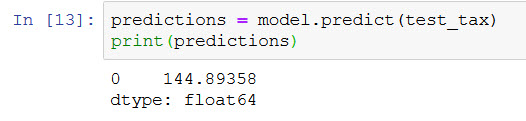
The result is 144.89358.
Using Statsmodels to Perform Multiple Linear Regression in Python
Working on the same dataset, let us now see if we get a better prediction by considering a combination of more than one input variables. Let’s try using a combination of ‘Taxes’, ‘Living’ and ‘List’ fields. Note that there may be more independent variables that account for the selling price, but for the time being let’s just go with these three.
Let’s create a new dataframe, new_X and assign the columns ‘Taxes’, Living’ and ‘List’ to it.
new_X = df[['Taxes','Living','List']]Don’t forget to convert the values to type float:
new_X=new_X.astype(float)You can also choose to add a constant value to the input distribution (This is optional, but you can try and see if it makes a difference to your ultimate result):
new_X = sm.add_constant(new_X)Create a new OLS model named ‘new_model’ and assign to it the variables new_X and Y. Apply the fit() function to find the ideal regression plane that fits the distribution of new_X and Y :
new_model = sm.OLS(Y,new_X).fit()The variable new_model now holds the detailed information about our fitted regression model. Let’s print the summary of our model results:
print(new_model.summary())Understanding the Results
Here’s a screenshot of the results we get:
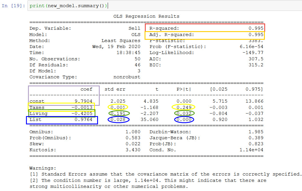
The first thing you’ll notice here is that there are now 4 different coefficient values instead of one. These are coefficients (or M values) corresponding to Taxes, Age and List. There’s also an additional coefficient called the constant coefficient, which is basically the C value in our regression equation.
Let us assimilate the significant values from this summary:
The R-squared value is 0.995. It’s a high value which means the regression plane fits quite well with the real data points.
Adj, R-squared is equal to the R-squared value, which is a good sign.
The constant coefficient value (C) is 9.7904
Now let’s take a look at each of the independent variables and how they affect the selling price.
- List price (or asking price) coefficient is 0.9764, which means the selling price is positively correlated to the asking price, which also makes sense intuitively. The corresponding p-value is also less than 0.05, further reinforcing the relationship.
- Interestingly, we see that the Living Area coefficient is -0.4205. This means that selling price decreases with increasing living area. The p-value for this is also less than 0.05, meaning that this variable has a significant effect on the selling price.
This may be explained by the fact that a higher living area leaves less area for other rooms, bringing the number of bedrooms, bathroom, etc. down. Maybe if we had included the Acres field, this result could have been easier to explain.
- Another point of interest is that we get a negative coefficient for Taxes (-0.0013), this is just the opposite of what we found out from our earlier model. The p-value for Taxes (0.249) tells us that of the three variables that we considered, Taxes have a low significance to the selling price.
Had we not considered the other variables, we would not have been able to see the full picture. This is why multiple regression analysis makes more sense in real-life applications.
Making Predictions
To see how close this regression plane is to our actual results, let’s use the predict() function, passing the whole dataframe of the input new_X to it.
predictions = new_model.predict(new_X)
print(predictions)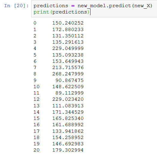
If you compare these predicted values you will find the results quite close to the original values of Selling Price. In fact, these results are actually closer to the original selling price values than when we used simple linear regression.
Relying on this model, let’s find our selling price for the following values:
- Taxes: 3200.0
- List: 165.0
- Living: 14.0
- Const: 1.0
(If you check the new_X values, you will find there’s an extra column labeled ‘const’, with a value 1.0. for all observations)
We need to make a dataframe with these four values.
test_input=pd.DataFrame({"const":[1.0], "Taxes":[3200.0], "Living":[14.0], "List":[165.0]})Let’s use the predict function to get predictions for Selling price based on these values.
predictions = new_model.predict(test_input)
print(predictions)
The result is 160.967981.
In other words, the predicted selling price for the given combination of variables is 160.97
Summary
We have so far looked at linear regression and how you can implement it using the Statsmodels Python library.
We have tried to explain:
- What Linear Regression is
- The difference between Simple and Multiple Linear Regression
- How to use Statsmodels to perform both Simple and Multiple Regression Analysis
When performing linear regression in Python, we need to follow the steps below:
- Install and import the packages needed.
- Get the dataset.
- Separate data into input and output variables.
- Use Statsmodels to create a regression model and fit it with the data.
- Get a summary of the result and interpret it to understand the relationships between variables
- Use the model to make predictions
For further reading you can take a look at some more examples in similar posts and resources:
- The Statsmodels official documentation on Using statsmodels for OLS estimation
- Linear Regression from the Statsmodels official documentation
- Predicting Housing Prices with Linear Regression using Python, pandas, and statsmodels from Learn Data Science
- Example of Multiple Linear Regression in Python from Data to Fish
The GitHub repo with the code snippets discussed in this article can be found here.